- Privacy Policy
Home » ANOVA (Analysis of variance) – Formulas, Types, and Examples

ANOVA (Analysis of variance) – Formulas, Types, and Examples
Table of Contents

Analysis of Variance (ANOVA)
Analysis of Variance (ANOVA) is a statistical method used to test differences between two or more means. It is similar to the t-test, but the t-test is generally used for comparing two means, while ANOVA is used when you have more than two means to compare.
ANOVA is based on comparing the variance (or variation) between the data samples to the variation within each particular sample. If the between-group variance is high and the within-group variance is low, this provides evidence that the means of the groups are significantly different.
ANOVA Terminology
When discussing ANOVA, there are several key terms to understand:
- Factor : This is another term for the independent variable in your analysis. In a one-way ANOVA, there is one factor, while in a two-way ANOVA, there are two factors.
- Levels : These are the different groups or categories within a factor. For example, if the factor is ‘diet’ the levels might be ‘low fat’, ‘medium fat’, and ‘high fat’.
- Response Variable : This is the dependent variable or the outcome that you are measuring.
- Within-group Variance : This is the variance or spread of scores within each level of your factor.
- Between-group Variance : This is the variance or spread of scores between the different levels of your factor.
- Grand Mean : This is the overall mean when you consider all the data together, regardless of the factor level.
- Treatment Sums of Squares (SS) : This represents the between-group variability. It is the sum of the squared differences between the group means and the grand mean.
- Error Sums of Squares (SS) : This represents the within-group variability. It’s the sum of the squared differences between each observation and its group mean.
- Total Sums of Squares (SS) : This is the sum of the Treatment SS and the Error SS. It represents the total variability in the data.
- Degrees of Freedom (df) : The degrees of freedom are the number of values that have the freedom to vary when computing a statistic. For example, if you have ‘n’ observations in one group, then the degrees of freedom for that group is ‘n-1’.
- Mean Square (MS) : Mean Square is the average squared deviation and is calculated by dividing the sum of squares by the corresponding degrees of freedom.
- F-Ratio : This is the test statistic for ANOVAs, and it’s the ratio of the between-group variance to the within-group variance. If the between-group variance is significantly larger than the within-group variance, the F-ratio will be large and likely significant.
- Null Hypothesis (H0) : This is the hypothesis that there is no difference between the group means.
- Alternative Hypothesis (H1) : This is the hypothesis that there is a difference between at least two of the group means.
- p-value : This is the probability of obtaining a test statistic as extreme as the one that was actually observed, assuming that the null hypothesis is true. If the p-value is less than the significance level (usually 0.05), then the null hypothesis is rejected in favor of the alternative hypothesis.
- Post-hoc tests : These are follow-up tests conducted after an ANOVA when the null hypothesis is rejected, to determine which specific groups’ means (levels) are different from each other. Examples include Tukey’s HSD, Scheffe, Bonferroni, among others.
Types of ANOVA
Types of ANOVA are as follows:
One-way (or one-factor) ANOVA
This is the simplest type of ANOVA, which involves one independent variable . For example, comparing the effect of different types of diet (vegetarian, pescatarian, omnivore) on cholesterol level.
Two-way (or two-factor) ANOVA
This involves two independent variables. This allows for testing the effect of each independent variable on the dependent variable , as well as testing if there’s an interaction effect between the independent variables on the dependent variable.
Repeated Measures ANOVA
This is used when the same subjects are measured multiple times under different conditions, or at different points in time. This type of ANOVA is often used in longitudinal studies.
Mixed Design ANOVA
This combines features of both between-subjects (independent groups) and within-subjects (repeated measures) designs. In this model, one factor is a between-subjects variable and the other is a within-subjects variable.
Multivariate Analysis of Variance (MANOVA)
This is used when there are two or more dependent variables. It tests whether changes in the independent variable(s) correspond to changes in the dependent variables.
Analysis of Covariance (ANCOVA)
This combines ANOVA and regression. ANCOVA tests whether certain factors have an effect on the outcome variable after removing the variance for which quantitative covariates (interval variables) account. This allows the comparison of one variable outcome between groups, while statistically controlling for the effect of other continuous variables that are not of primary interest.
Nested ANOVA
This model is used when the groups can be clustered into categories. For example, if you were comparing students’ performance from different classrooms and different schools, “classroom” could be nested within “school.”
ANOVA Formulas
ANOVA Formulas are as follows:
Sum of Squares Total (SST)
This represents the total variability in the data. It is the sum of the squared differences between each observation and the overall mean.
- yi represents each individual data point
- y_mean represents the grand mean (mean of all observations)
Sum of Squares Within (SSW)
This represents the variability within each group or factor level. It is the sum of the squared differences between each observation and its group mean.
- yij represents each individual data point within a group
- y_meani represents the mean of the ith group
Sum of Squares Between (SSB)
This represents the variability between the groups. It is the sum of the squared differences between the group means and the grand mean, multiplied by the number of observations in each group.
- ni represents the number of observations in each group
- y_mean represents the grand mean
Degrees of Freedom
The degrees of freedom are the number of values that have the freedom to vary when calculating a statistic.
For within groups (dfW):
For between groups (dfB):
For total (dfT):
- N represents the total number of observations
- k represents the number of groups
Mean Squares
Mean squares are the sum of squares divided by the respective degrees of freedom.
Mean Squares Between (MSB):
Mean Squares Within (MSW):
F-Statistic
The F-statistic is used to test whether the variability between the groups is significantly greater than the variability within the groups.
If the F-statistic is significantly higher than what would be expected by chance, we reject the null hypothesis that all group means are equal.
Examples of ANOVA
Examples 1:
Suppose a psychologist wants to test the effect of three different types of exercise (yoga, aerobic exercise, and weight training) on stress reduction. The dependent variable is the stress level, which can be measured using a stress rating scale.
Here are hypothetical stress ratings for a group of participants after they followed each of the exercise regimes for a period:
- Yoga: [3, 2, 2, 1, 2, 2, 3, 2, 1, 2]
- Aerobic Exercise: [2, 3, 3, 2, 3, 2, 3, 3, 2, 2]
- Weight Training: [4, 4, 5, 5, 4, 5, 4, 5, 4, 5]
The psychologist wants to determine if there is a statistically significant difference in stress levels between these different types of exercise.
To conduct the ANOVA:
1. State the hypotheses:
- Null Hypothesis (H0): There is no difference in mean stress levels between the three types of exercise.
- Alternative Hypothesis (H1): There is a difference in mean stress levels between at least two of the types of exercise.
2. Calculate the ANOVA statistics:
- Compute the Sum of Squares Between (SSB), Sum of Squares Within (SSW), and Sum of Squares Total (SST).
- Calculate the Degrees of Freedom (dfB, dfW, dfT).
- Calculate the Mean Squares Between (MSB) and Mean Squares Within (MSW).
- Compute the F-statistic (F = MSB / MSW).
3. Check the p-value associated with the calculated F-statistic.
- If the p-value is less than the chosen significance level (often 0.05), then we reject the null hypothesis in favor of the alternative hypothesis. This suggests there is a statistically significant difference in mean stress levels between the three exercise types.
4. Post-hoc tests
- If we reject the null hypothesis, we conduct a post-hoc test to determine which specific groups’ means (exercise types) are different from each other.
Examples 2:
Suppose an agricultural scientist wants to compare the yield of three varieties of wheat. The scientist randomly selects four fields for each variety and plants them. After harvest, the yield from each field is measured in bushels. Here are the hypothetical yields:
The scientist wants to know if the differences in yields are due to the different varieties or just random variation.
Here’s how to apply the one-way ANOVA to this situation:
- Null Hypothesis (H0): The means of the three populations are equal.
- Alternative Hypothesis (H1): At least one population mean is different.
- Calculate the Degrees of Freedom (dfB for between groups, dfW for within groups, dfT for total).
- If the p-value is less than the chosen significance level (often 0.05), then we reject the null hypothesis in favor of the alternative hypothesis. This would suggest there is a statistically significant difference in mean yields among the three varieties.
- If we reject the null hypothesis, we conduct a post-hoc test to determine which specific groups’ means (wheat varieties) are different from each other.
How to Conduct ANOVA
Conducting an Analysis of Variance (ANOVA) involves several steps. Here’s a general guideline on how to perform it:
- Null Hypothesis (H0): The means of all groups are equal.
- Alternative Hypothesis (H1): At least one group mean is different from the others.
- The significance level (often denoted as α) is usually set at 0.05. This implies that you are willing to accept a 5% chance that you are wrong in rejecting the null hypothesis.
- Data should be collected for each group under study. Make sure that the data meet the assumptions of an ANOVA: normality, independence, and homogeneity of variances.
- Calculate the Degrees of Freedom (df) for each sum of squares (dfB, dfW, dfT).
- Compute the Mean Squares Between (MSB) and Mean Squares Within (MSW) by dividing the sum of squares by the corresponding degrees of freedom.
- Compute the F-statistic as the ratio of MSB to MSW.
- Determine the critical F-value from the F-distribution table using dfB and dfW.
- If the calculated F-statistic is greater than the critical F-value, reject the null hypothesis.
- If the p-value associated with the calculated F-statistic is smaller than the significance level (0.05 typically), you reject the null hypothesis.
- If you rejected the null hypothesis, you can conduct post-hoc tests (like Tukey’s HSD) to determine which specific groups’ means (if you have more than two groups) are different from each other.
- Regardless of the result, report your findings in a clear, understandable manner. This typically includes reporting the test statistic, p-value, and whether the null hypothesis was rejected.
When to use ANOVA
ANOVA (Analysis of Variance) is used when you have three or more groups and you want to compare their means to see if they are significantly different from each other. It is a statistical method that is used in a variety of research scenarios. Here are some examples of when you might use ANOVA:
- Comparing Groups : If you want to compare the performance of more than two groups, for example, testing the effectiveness of different teaching methods on student performance.
- Evaluating Interactions : In a two-way or factorial ANOVA, you can test for an interaction effect. This means you are not only interested in the effect of each individual factor, but also whether the effect of one factor depends on the level of another factor.
- Repeated Measures : If you have measured the same subjects under different conditions or at different time points, you can use repeated measures ANOVA to compare the means of these repeated measures while accounting for the correlation between measures from the same subject.
- Experimental Designs : ANOVA is often used in experimental research designs when subjects are randomly assigned to different conditions and the goal is to compare the means of the conditions.
Here are the assumptions that must be met to use ANOVA:
- Normality : The data should be approximately normally distributed.
- Homogeneity of Variances : The variances of the groups you are comparing should be roughly equal. This assumption can be tested using Levene’s test or Bartlett’s test.
- Independence : The observations should be independent of each other. This assumption is met if the data is collected appropriately with no related groups (e.g., twins, matched pairs, repeated measures).
Applications of ANOVA
The Analysis of Variance (ANOVA) is a powerful statistical technique that is used widely across various fields and industries. Here are some of its key applications:
Agriculture
ANOVA is commonly used in agricultural research to compare the effectiveness of different types of fertilizers, crop varieties, or farming methods. For example, an agricultural researcher could use ANOVA to determine if there are significant differences in the yields of several varieties of wheat under the same conditions.
Manufacturing and Quality Control
ANOVA is used to determine if different manufacturing processes or machines produce different levels of product quality. For instance, an engineer might use it to test whether there are differences in the strength of a product based on the machine that produced it.
Marketing Research
Marketers often use ANOVA to test the effectiveness of different advertising strategies. For example, a marketer could use ANOVA to determine whether different marketing messages have a significant impact on consumer purchase intentions.
Healthcare and Medicine
In medical research, ANOVA can be used to compare the effectiveness of different treatments or drugs. For example, a medical researcher could use ANOVA to test whether there are significant differences in recovery times for patients who receive different types of therapy.
ANOVA is used in educational research to compare the effectiveness of different teaching methods or educational interventions. For example, an educator could use it to test whether students perform significantly differently when taught with different teaching methods.
Psychology and Social Sciences
Psychologists and social scientists use ANOVA to compare group means on various psychological and social variables. For example, a psychologist could use it to determine if there are significant differences in stress levels among individuals in different occupations.
Biology and Environmental Sciences
Biologists and environmental scientists use ANOVA to compare different biological and environmental conditions. For example, an environmental scientist could use it to determine if there are significant differences in the levels of a pollutant in different bodies of water.
Advantages of ANOVA
Here are some advantages of using ANOVA:
Comparing Multiple Groups: One of the key advantages of ANOVA is the ability to compare the means of three or more groups. This makes it more powerful and flexible than the t-test, which is limited to comparing only two groups.
Control of Type I Error: When comparing multiple groups, the chances of making a Type I error (false positive) increases. One of the strengths of ANOVA is that it controls the Type I error rate across all comparisons. This is in contrast to performing multiple pairwise t-tests which can inflate the Type I error rate.
Testing Interactions: In factorial ANOVA, you can test not only the main effect of each factor, but also the interaction effect between factors. This can provide valuable insights into how different factors or variables interact with each other.
Handling Continuous and Categorical Variables: ANOVA can handle both continuous and categorical variables . The dependent variable is continuous and the independent variables are categorical.
Robustness: ANOVA is considered robust to violations of normality assumption when group sizes are equal. This means that even if your data do not perfectly meet the normality assumption, you might still get valid results.
Provides Detailed Analysis: ANOVA provides a detailed breakdown of variances and interactions between variables which can be useful in understanding the underlying factors affecting the outcome.
Capability to Handle Complex Experimental Designs: Advanced types of ANOVA (like repeated measures ANOVA, MANOVA, etc.) can handle more complex experimental designs, including those where measurements are taken on the same subjects over time, or when you want to analyze multiple dependent variables at once.
Disadvantages of ANOVA
Some limitations or disadvantages that are important to consider:
Assumptions: ANOVA relies on several assumptions including normality (the data follows a normal distribution), independence (the observations are independent of each other), and homogeneity of variances (the variances of the groups are roughly equal). If these assumptions are violated, the results of the ANOVA may not be valid.
Sensitivity to Outliers: ANOVA can be sensitive to outliers. A single extreme value in one group can affect the sum of squares and consequently influence the F-statistic and the overall result of the test.
Dichotomous Variables: ANOVA is not suitable for dichotomous variables (variables that can take only two values, like yes/no or male/female). It is used to compare the means of groups for a continuous dependent variable.
Lack of Specificity: Although ANOVA can tell you that there is a significant difference between groups, it doesn’t tell you which specific groups are significantly different from each other. You need to carry out further post-hoc tests (like Tukey’s HSD or Bonferroni) for these pairwise comparisons.
Complexity with Multiple Factors: When dealing with multiple factors and interactions in factorial ANOVA, interpretation can become complex. The presence of interaction effects can make main effects difficult to interpret.
Requires Larger Sample Sizes: To detect an effect of a certain size, ANOVA generally requires larger sample sizes than a t-test.
Equal Group Sizes: While not always a strict requirement, ANOVA is most powerful and its assumptions are most likely to be met when groups are of equal or similar sizes.
About the author

Muhammad Hassan
Researcher, Academic Writer, Web developer
You may also like

Content Analysis – Methods, Types and Examples

Documentary Analysis – Methods, Applications and...

Narrative Analysis – Types, Methods and Examples

Graphical Methods – Types, Examples and Guide

Substantive Framework – Types, Methods and...

Inferential Statistics – Types, Methods and...
Have a language expert improve your writing
Run a free plagiarism check in 10 minutes, generate accurate citations for free.
- Knowledge Base
One-way ANOVA | When and How to Use It (With Examples)
Published on March 6, 2020 by Rebecca Bevans . Revised on May 10, 2024.
ANOVA , which stands for Analysis of Variance, is a statistical test used to analyze the difference between the means of more than two groups.
A one-way ANOVA uses one independent variable , while a two-way ANOVA uses two independent variables.
Table of contents
When to use a one-way anova, how does an anova test work, assumptions of anova, performing a one-way anova, interpreting the results, post-hoc testing, reporting the results of anova, other interesting articles, frequently asked questions about one-way anova.
Use a one-way ANOVA when you have collected data about one categorical independent variable and one quantitative dependent variable . The independent variable should have at least three levels (i.e. at least three different groups or categories).
ANOVA tells you if the dependent variable changes according to the level of the independent variable. For example:
- Your independent variable is social media use , and you assign groups to low , medium , and high levels of social media use to find out if there is a difference in hours of sleep per night .
- Your independent variable is brand of soda , and you collect data on Coke , Pepsi , Sprite , and Fanta to find out if there is a difference in the price per 100ml .
- You independent variable is type of fertilizer , and you treat crop fields with mixtures 1 , 2 and 3 to find out if there is a difference in crop yield .
The null hypothesis ( H 0 ) of ANOVA is that there is no difference among group means. The alternative hypothesis ( H a ) is that at least one group differs significantly from the overall mean of the dependent variable.
If you only want to compare two groups, use a t test instead.
Prevent plagiarism. Run a free check.
ANOVA determines whether the groups created by the levels of the independent variable are statistically different by calculating whether the means of the treatment levels are different from the overall mean of the dependent variable.
If any of the group means is significantly different from the overall mean, then the null hypothesis is rejected.
ANOVA uses the F test for statistical significance . This allows for comparison of multiple means at once, because the error is calculated for the whole set of comparisons rather than for each individual two-way comparison (which would happen with a t test).
The F test compares the variance in each group mean from the overall group variance. If the variance within groups is smaller than the variance between groups , the F test will find a higher F value, and therefore a higher likelihood that the difference observed is real and not due to chance.
The assumptions of the ANOVA test are the same as the general assumptions for any parametric test:
- Independence of observations : the data were collected using statistically valid sampling methods , and there are no hidden relationships among observations. If your data fail to meet this assumption because you have a confounding variable that you need to control for statistically, use an ANOVA with blocking variables.
- Normally-distributed response variable : The values of the dependent variable follow a normal distribution .
- Homogeneity of variance : The variation within each group being compared is similar for every group. If the variances are different among the groups, then ANOVA probably isn’t the right fit for the data.
While you can perform an ANOVA by hand , it is difficult to do so with more than a few observations. We will perform our analysis in the R statistical program because it is free, powerful, and widely available. For a full walkthrough of this ANOVA example, see our guide to performing ANOVA in R .
The sample dataset from our imaginary crop yield experiment contains data about:
- fertilizer type (type 1, 2, or 3)
- planting density (1 = low density, 2 = high density)
- planting location in the field (blocks 1, 2, 3, or 4)
- final crop yield (in bushels per acre).
This gives us enough information to run various different ANOVA tests and see which model is the best fit for the data.
For the one-way ANOVA, we will only analyze the effect of fertilizer type on crop yield.
Sample dataset for ANOVA
After loading the dataset into our R environment, we can use the command aov() to run an ANOVA. In this example we will model the differences in the mean of the response variable , crop yield, as a function of type of fertilizer.
To view the summary of a statistical model in R, use the summary() function.
The summary of an ANOVA test (in R) looks like this:

The ANOVA output provides an estimate of how much variation in the dependent variable that can be explained by the independent variable.
- The first column lists the independent variable along with the model residuals (aka the model error).
- The Df column displays the degrees of freedom for the independent variable (calculated by taking the number of levels within the variable and subtracting 1), and the degrees of freedom for the residuals (calculated by taking the total number of observations minus 1, then subtracting the number of levels in each of the independent variables).
- The Sum Sq column displays the sum of squares (a.k.a. the total variation) between the group means and the overall mean explained by that variable. The sum of squares for the fertilizer variable is 6.07, while the sum of squares of the residuals is 35.89.
- The Mean Sq column is the mean of the sum of squares, which is calculated by dividing the sum of squares by the degrees of freedom.
- The F value column is the test statistic from the F test: the mean square of each independent variable divided by the mean square of the residuals. The larger the F value, the more likely it is that the variation associated with the independent variable is real and not due to chance.
- The Pr(>F) column is the p value of the F statistic. This shows how likely it is that the F value calculated from the test would have occurred if the null hypothesis of no difference among group means were true.
Because the p value of the independent variable, fertilizer, is statistically significant ( p < 0.05), it is likely that fertilizer type does have a significant effect on average crop yield.
ANOVA will tell you if there are differences among the levels of the independent variable, but not which differences are significant. To find how the treatment levels differ from one another, perform a TukeyHSD (Tukey’s Honestly-Significant Difference) post-hoc test.
The Tukey test runs pairwise comparisons among each of the groups, and uses a conservative error estimate to find the groups which are statistically different from one another.
The output of the TukeyHSD looks like this:

First, the table reports the model being tested (‘Fit’). Next it lists the pairwise differences among groups for the independent variable.
Under the ‘$fertilizer’ section, we see the mean difference between each fertilizer treatment (‘diff’), the lower and upper bounds of the 95% confidence interval (‘lwr’ and ‘upr’), and the p value , adjusted for multiple pairwise comparisons.
The pairwise comparisons show that fertilizer type 3 has a significantly higher mean yield than both fertilizer 2 and fertilizer 1, but the difference between the mean yields of fertilizers 2 and 1 is not statistically significant.
When reporting the results of an ANOVA, include a brief description of the variables you tested, the F value, degrees of freedom, and p values for each independent variable, and explain what the results mean.
If you want to provide more detailed information about the differences found in your test, you can also include a graph of the ANOVA results , with grouping letters above each level of the independent variable to show which groups are statistically different from one another:

If you want to know more about statistics , methodology , or research bias , make sure to check out some of our other articles with explanations and examples.
- Chi square test of independence
- Statistical power
- Descriptive statistics
- Degrees of freedom
- Pearson correlation
- Null hypothesis
Methodology
- Double-blind study
- Case-control study
- Research ethics
- Data collection
- Hypothesis testing
- Structured interviews
Research bias
- Hawthorne effect
- Unconscious bias
- Recall bias
- Halo effect
- Self-serving bias
- Information bias
The only difference between one-way and two-way ANOVA is the number of independent variables . A one-way ANOVA has one independent variable, while a two-way ANOVA has two.
- One-way ANOVA : Testing the relationship between shoe brand (Nike, Adidas, Saucony, Hoka) and race finish times in a marathon.
- Two-way ANOVA : Testing the relationship between shoe brand (Nike, Adidas, Saucony, Hoka), runner age group (junior, senior, master’s), and race finishing times in a marathon.
All ANOVAs are designed to test for differences among three or more groups. If you are only testing for a difference between two groups, use a t-test instead.
A factorial ANOVA is any ANOVA that uses more than one categorical independent variable . A two-way ANOVA is a type of factorial ANOVA.
Some examples of factorial ANOVAs include:
- Testing the combined effects of vaccination (vaccinated or not vaccinated) and health status (healthy or pre-existing condition) on the rate of flu infection in a population.
- Testing the effects of marital status (married, single, divorced, widowed), job status (employed, self-employed, unemployed, retired), and family history (no family history, some family history) on the incidence of depression in a population.
- Testing the effects of feed type (type A, B, or C) and barn crowding (not crowded, somewhat crowded, very crowded) on the final weight of chickens in a commercial farming operation.
In ANOVA, the null hypothesis is that there is no difference among group means. If any group differs significantly from the overall group mean, then the ANOVA will report a statistically significant result.
Significant differences among group means are calculated using the F statistic, which is the ratio of the mean sum of squares (the variance explained by the independent variable) to the mean square error (the variance left over).
If the F statistic is higher than the critical value (the value of F that corresponds with your alpha value, usually 0.05), then the difference among groups is deemed statistically significant.
Quantitative variables are any variables where the data represent amounts (e.g. height, weight, or age).
Categorical variables are any variables where the data represent groups. This includes rankings (e.g. finishing places in a race), classifications (e.g. brands of cereal), and binary outcomes (e.g. coin flips).
You need to know what type of variables you are working with to choose the right statistical test for your data and interpret your results .
Cite this Scribbr article
If you want to cite this source, you can copy and paste the citation or click the “Cite this Scribbr article” button to automatically add the citation to our free Citation Generator.
Bevans, R. (2024, May 09). One-way ANOVA | When and How to Use It (With Examples). Scribbr. Retrieved September 3, 2024, from https://www.scribbr.com/statistics/one-way-anova/
Is this article helpful?

Rebecca Bevans
Other students also liked, two-way anova | examples & when to use it, anova in r | a complete step-by-step guide with examples, guide to experimental design | overview, steps, & examples, what is your plagiarism score.
ANOVA Test: Definition, Types, Examples, SPSS
Statistics Definitions > ANOVA Contents :
The ANOVA Test
- How to Run a One Way ANOVA in SPSS
Two Way ANOVA
What is manova, what is factorial anova, how to run an anova, anova vs. t test.
- Repeated Measures ANOVA in SPSS: Steps
Related Articles
Watch the video for an introduction to ANOVA.

Can’t see the video? Click here to watch it on YouTube.
An ANOVA test is a way to find out if survey or experiment results are significant . In other words, they help you to figure out if you need to reject the null hypothesis or accept the alternate hypothesis .
Basically, you’re testing groups to see if there’s a difference between them. Examples of when you might want to test different groups:
- A group of psychiatric patients are trying three different therapies: counseling, medication and biofeedback. You want to see if one therapy is better than the others.
- A manufacturer has two different processes to make light bulbs. They want to know if one process is better than the other.
- Students from different colleges take the same exam. You want to see if one college outperforms the other.
What Does “One-Way” or “Two-Way Mean?
One-way or two-way refers to the number of independent variables (IVs) in your Analysis of Variance test.
- One-way has one independent variable (with 2 levels ). For example: brand of cereal ,
- Two-way has two independent variables (it can have multiple levels). For example: brand of cereal, calories .
What are “Groups” or “Levels”?
Groups or levels are different groups within the same independent variable . In the above example, your levels for “brand of cereal” might be Lucky Charms, Raisin Bran, Cornflakes — a total of three levels. Your levels for “Calories” might be: sweetened, unsweetened — a total of two levels.
Let’s say you are studying if an alcoholic support group and individual counseling combined is the most effective treatment for lowering alcohol consumption. You might split the study participants into three groups or levels:
- Medication only,
- Medication and counseling,
- Counseling only.
Your dependent variable would be the number of alcoholic beverages consumed per day.
If your groups or levels have a hierarchical structure (each level has unique subgroups), then use a nested ANOVA for the analysis.
What Does “Replication” Mean?
It’s whether you are replicating (i.e. duplicating) your test(s) with multiple groups. With a two way ANOVA with replication , you have two groups and individuals within that group are doing more than one thing (i.e. two groups of students from two colleges taking two tests). If you only have one group taking two tests, you would use without replication.
Types of Tests.
There are two main types: one-way and two-way. Two-way tests can be with or without replication.
- One-way ANOVA between groups: used when you want to test two groups to see if there’s a difference between them.
- Two way ANOVA without replication: used when you have one group and you’re double-testing that same group. For example, you’re testing one set of individuals before and after they take a medication to see if it works or not.
- Two way ANOVA with replication: Two groups , and the members of those groups are doing more than one thing . For example, two groups of patients from different hospitals trying two different therapies.
Back to Top
One Way ANOVA
A one way ANOVA is used to compare two means from two independent (unrelated) groups using the F-distribution . The null hypothesis for the test is that the two means are equal. Therefore, a significant result means that the two means are unequal.
Examples of when to use a one way ANOVA
Situation 1: You have a group of individuals randomly split into smaller groups and completing different tasks. For example, you might be studying the effects of tea on weight loss and form three groups: green tea, black tea, and no tea. Situation 2: Similar to situation 1, but in this case the individuals are split into groups based on an attribute they possess. For example, you might be studying leg strength of people according to weight. You could split participants into weight categories (obese, overweight and normal) and measure their leg strength on a weight machine.
Limitations of the One Way ANOVA
A one way ANOVA will tell you that at least two groups were different from each other. But it won’t tell you which groups were different. If your test returns a significant f-statistic, you may need to run an ad hoc test (like the Least Significant Difference test) to tell you exactly which groups had a difference in means . Back to Top
How to run a One Way ANOVA in SPSS

A Two Way ANOVA is an extension of the One Way ANOVA. With a One Way, you have one independent variable affecting a dependent variable . With a Two Way ANOVA, there are two independents. Use a two way ANOVA when you have one measurement variable (i.e. a quantitative variable ) and two nominal variables . In other words, if your experiment has a quantitative outcome and you have two categorical explanatory variables , a two way ANOVA is appropriate.
For example, you might want to find out if there is an interaction between income and gender for anxiety level at job interviews. The anxiety level is the outcome, or the variable that can be measured. Gender and Income are the two categorical variables . These categorical variables are also the independent variables, which are called factors in a Two Way ANOVA.
The factors can be split into levels . In the above example, income level could be split into three levels: low, middle and high income. Gender could be split into three levels: male, female, and transgender. Treatment groups are all possible combinations of the factors. In this example there would be 3 x 3 = 9 treatment groups.
Main Effect and Interaction Effect
The results from a Two Way ANOVA will calculate a main effect and an interaction effect . The main effect is similar to a One Way ANOVA: each factor’s effect is considered separately. With the interaction effect, all factors are considered at the same time. Interaction effects between factors are easier to test if there is more than one observation in each cell. For the above example, multiple stress scores could be entered into cells. If you do enter multiple observations into cells, the number in each cell must be equal.
Two null hypotheses are tested if you are placing one observation in each cell. For this example, those hypotheses would be: H 01 : All the income groups have equal mean stress. H 02 : All the gender groups have equal mean stress.
For multiple observations in cells, you would also be testing a third hypothesis: H 03 : The factors are independent or the interaction effect does not exist.
An F-statistic is computed for each hypothesis you are testing.
Assumptions for Two Way ANOVA
- The population must be close to a normal distribution .
- Samples must be independent.
- Population variances must be equal (i.e. homoscedastic ).
- Groups must have equal sample sizes .
MANOVA is just an ANOVA with several dependent variables. It’s similar to many other tests and experiments in that it’s purpose is to find out if the response variable (i.e. your dependent variable) is changed by manipulating the independent variable. The test helps to answer many research questions, including:
- Do changes to the independent variables have statistically significant effects on dependent variables?
- What are the interactions among dependent variables?
- What are the interactions among independent variables?
MANOVA Example
Suppose you wanted to find out if a difference in textbooks affected students’ scores in math and science. Improvements in math and science means that there are two dependent variables, so a MANOVA is appropriate.
An ANOVA will give you a single ( univariate ) f-value while a MANOVA will give you a multivariate F value. MANOVA tests the multiple dependent variables by creating new, artificial, dependent variables that maximize group differences. These new dependent variables are linear combinations of the measured dependent variables.
Interpreting the MANOVA results
If the multivariate F value indicates the test is statistically significant , this means that something is significant. In the above example, you would not know if math scores have improved, science scores have improved (or both). Once you have a significant result, you would then have to look at each individual component (the univariate F tests) to see which dependent variable(s) contributed to the statistically significant result.
Advantages and Disadvantages of MANOVA vs. ANOVA
- MANOVA enables you to test multiple dependent variables.
- MANOVA can protect against Type I errors.
Disadvantages
- MANOVA is many times more complicated than ANOVA, making it a challenge to see which independent variables are affecting dependent variables.
- One degree of freedom is lost with the addition of each new variable .
- The dependent variables should be uncorrelated as much as possible. If they are correlated, the loss in degrees of freedom means that there isn’t much advantages in including more than one dependent variable on the test.
Reference : SFSU. Retrieved April 18, 2022 from: http://online.sfsu.edu/efc/classes/biol710/manova/MANOVAnewest.pdf
A factorial ANOVA is an Analysis of Variance test with more than one independent variable , or “ factor “. It can also refer to more than one Level of Independent Variable . For example, an experiment with a treatment group and a control group has one factor (the treatment) but two levels (the treatment and the control). The terms “two-way” and “three-way” refer to the number of factors or the number of levels in your test. Four-way ANOVA and above are rarely used because the results of the test are complex and difficult to interpret.
- A two-way ANOVA has two factors ( independent variables ) and one dependent variable . For example, time spent studying and prior knowledge are factors that affect how well you do on a test.
- A three-way ANOVA has three factors (independent variables) and one dependent variable. For example, time spent studying, prior knowledge, and hours of sleep are factors that affect how well you do on a test
Factorial ANOVA is an efficient way of conducting a test. Instead of performing a series of experiments where you test one independent variable against one dependent variable, you can test all independent variables at the same time.
Variability
In a one-way ANOVA, variability is due to the differences between groups and the differences within groups. In factorial ANOVA, each level and factor are paired up with each other (“crossed”). This helps you to see what interactions are going on between the levels and factors. If there is an interaction then the differences in one factor depend on the differences in another.
Let’s say you were running a two-way ANOVA to test male/female performance on a final exam. The subjects had either had 4, 6, or 8 hours of sleep.
- IV1: SEX (Male/Female)
- IV2: SLEEP (4/6/8)
- DV: Final Exam Score
A two-way factorial ANOVA would help you answer the following questions:
- Is sex a main effect? In other words, do men and women differ significantly on their exam performance?
- Is sleep a main effect? In other words, do people who have had 4,6, or 8 hours of sleep differ significantly in their performance?
- Is there a significant interaction between factors? In other words, how do hours of sleep and sex interact with regards to exam performance?
- Can any differences in sex and exam performance be found in the different levels of sleep?
Assumptions of Factorial ANOVA
- Normality: the dependent variable is normally distributed.
- Independence: Observations and groups are independent from each other.
- Equality of Variance: the population variances are equal across factors/levels.
These tests are very time-consuming by hand. In nearly every case you’ll want to use software. For example, several options are available in Excel :
- Two way ANOVA in Excel with replication and without replication.
- One way ANOVA in Excel 2013 .

ANOVA tests in statistics packages are run on parametric data. If you have rank or ordered data, you’ll want to run a non-parametric ANOVA (usually found under a different heading in the software, like “ nonparametric tests “).
It is unlikely you’ll want to do this test by hand, but if you must, these are the steps you’ll want to take:
- Find the mean for each of the groups.
- Find the overall mean (the mean of the groups combined).
- Find the Within Group Variation ; the total deviation of each member’s score from the Group Mean.
- Find the Between Group Variation : the deviation of each Group Mean from the Overall Mean.
- Find the F statistic: the ratio of Between Group Variation to Within Group Variation.
A Student’s t-test will tell you if there is a significant variation between groups. A t-test compares means, while the ANOVA compares variances between populations. You could technically perform a series of t-tests on your data. However, as the groups grow in number, you may end up with a lot of pair comparisons that you need to run. ANOVA will give you a single number (the f-statistic ) and one p-value to help you support or reject the null hypothesis . Back to Top
Repeated Measures (Within Subjects) ANOVA
A repeated measures ANOVA is almost the same as one-way ANOVA, with one main difference: you test related groups, not independent ones.
It’s called Repeated Measures because the same group of participants is being measured over and over again. For example, you could be studying the cholesterol levels of the same group of patients at 1, 3, and 6 months after changing their diet. For this example, the independent variable is “time” and the dependent variable is “cholesterol.” The independent variable is usually called the within-subjects factor .
Repeated measures ANOVA is similar to a simple multivariate design. In both tests, the same participants are measured over and over. However, with repeated measures the same characteristic is measured with a different condition. For example, blood pressure is measured over the condition “time”. For simple multivariate design it is the characteristic that changes. For example, you could measure blood pressure, heart rate and respiration rate over time.
Reasons to use Repeated Measures ANOVA
- When you collect data from the same participants over a period of time, individual differences (a source of between group differences) are reduced or eliminated.
- Testing is more powerful because the sample size isn’t divided between groups.
- The test can be economical, as you’re using the same participants.
Assumptions for Repeated Measures ANOVA
The results from your repeated measures ANOVA will be valid only if the following assumptions haven’t been violated:
- There must be one independent variable and one dependent variable.
- The dependent variable must be a continuous variable , on an interval scale or a ratio scale .
- The independent variable must be categorical , either on the nominal scale or ordinal scale.
- Ideally, levels of dependence between pairs of groups is equal (“sphericity”). Corrections are possible if this assumption is violated.
One Way Repeated Measures ANOVA in SPSS: Steps
Watch the video for the steps:

Step 2: Replace the “factor1” name with something that represents your independent variable. For example, you could put “age” or “time.”
Step 3: Enter the “Number of Levels.” This is how many times the dependent variable has been measured. For example, if you took measurements every week for a total of 4 weeks, this number would be 4.
Step 4: Click the “Add” button and then give your dependent variable a name.

Step 7: Click “Plots” and use the arrow keys to transfer the factor from the left box onto the Horizontal Axis box.

Step 9: Click “Options”, then transfer your factors from the left box to the Display Means for box on the right.
Step 10: Click the following check boxes:
- Compare main effects.
- Descriptive Statistics.
- Estimates of Effect Size .
Step 11: Select “Bonferroni” from the drop down menu under Confidence Interval Adjustment . Step 12: Click “Continue” and then click “OK” to run the test. Back to Top
In statistics, sphericity (ε) refers to Mauchly’s sphericity test , which was developed in 1940 by John W. Mauchly , who co-developed the first general-purpose electronic computer.
Sphericity is used as an assumption in repeated measures ANOVA. The assumption states that the variances of the differences between all possible group pairs are equal. If your data violates this assumption, it can result in an increase in a Type I error (the incorrect rejection of the null hypothesis) .
It’s very common for repeated measures ANOVA to result in a violation of the assumption. If the assumption has been violated, corrections have been developed that can avoid increases in the type I error rate. The correction is applied to the degrees of freedom in the F-distribution .
Mauchly’s Sphericity Test
Mauchly’s test for sphericity can be run in the majority of statistical software, where it tends to be the default test for sphericity. Mauchly’s test is ideal for mid-size samples. It may fail to detect sphericity in small samples and it may over-detect in large samples. If the test returns a small p-value (p ≤.05), this is an indication that your data has violated the assumption. The following picture of SPSS output for ANOVA shows that the significance “sig” attached to Mauchly’s is .274. This means that the assumption has not been violated for this set of data.
You would report the above result as “Mauchly’s Test indicated that the assumption of sphericity had not been violated, χ 2 (2) = 2.588, p = .274.”
If your test returned a small p-value , you should apply a correction, usually either the:
- Greehouse-Geisser correction.
- Huynh-Feldt correction .
When ε ≤ 0.75 (or you don’t know what the value for the statistic is), use the Greenhouse-Geisser correction. When ε > .75, use the Huynh-Feldt correction .
Grand mean ANOVA vs Regression
Blokdyk, B. (2018). Ad Hoc Testing . 5STARCooks Miller, R. G. Beyond ANOVA: Basics of Applied Statistics . Boca Raton, FL: Chapman & Hall, 1997 Image: UVM. Retrieved December 4, 2020 from: https://www.uvm.edu/~dhowell/gradstat/psych341/lectures/RepeatedMeasures/repeated1.html
An open portfolio of interoperable, industry leading products
The Dotmatics digital science platform provides the first true end-to-end solution for scientific R&D, combining an enterprise data platform with the most widely used applications for data analysis, biologics, flow cytometry, chemicals innovation, and more.

Statistical analysis and graphing software for scientists
Bioinformatics, cloning, and antibody discovery software
Plan, visualize, & document core molecular biology procedures
Electronic Lab Notebook to organize, search and share data
Proteomics software for analysis of mass spec data
Modern cytometry analysis platform
Analysis, statistics, graphing and reporting of flow cytometry data
Software to optimize designs of clinical trials
POPULAR USE CASES
The Ultimate Guide to ANOVA
Get all of your ANOVA questions answered here
ANOVA is the go-to analysis tool for classical experimental design, which forms the backbone of scientific research.
In this article, we’ll guide you through what ANOVA is, how to determine which version to use to evaluate your particular experiment, and provide detailed examples for the most common forms of ANOVA.
This includes a (brief) discussion of crossed, nested, fixed and random factors, and covers the majority of ANOVA models that a scientist would encounter before requiring the assistance of a statistician or modeling expert.
What is ANOVA used for?
ANOVA, or (Fisher’s) analysis of variance, is a critical analytical technique for evaluating differences between three or more sample means from an experiment. As the name implies, it partitions out the variance in the response variable based on one or more explanatory factors.
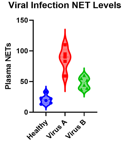
As you will see there are many types of ANOVA such as one-, two-, and three-way ANOVA as well as nested and repeated measures ANOVA. The graphic below shows a simple example of an experiment that requires ANOVA in which researchers measured the levels of neutrophil extracellular traps (NETs) in plasma across patients with different viral respiratory infections.
Many researchers may not realize that, for the majority of experiments, the characteristics of the experiment that you run dictate the ANOVA that you need to use to test the results. While it’s a massive topic (with professional training needed for some of the advanced techniques), this is a practical guide covering what most researchers need to know about ANOVA.
When should I use ANOVA?
If your response variable is numeric, and you’re looking for how that number differs across several categorical groups, then ANOVA is an ideal place to start. After running an experiment, ANOVA is used to analyze whether there are differences between the mean response of one or more of these grouping factors.
ANOVA can handle a large variety of experimental factors such as repeated measures on the same experimental unit (e.g., before/during/after).
If instead of evaluating treatment differences, you want to develop a model using a set of numeric variables to predict that numeric response variable, see linear regression and t tests .
What is the difference between one-way, two-way and three-way ANOVA?
The number of “ways” in ANOVA (e.g., one-way, two-way, …) is simply the number of factors in your experiment.
Although the difference in names sounds trivial, the complexity of ANOVA increases greatly with each added factor. To use an example from agriculture, let’s say we have designed an experiment to research how different factors influence the yield of a crop.
An experiment with a single factor
In the most basic version, we want to evaluate three different fertilizers. Because we have more than two groups, we have to use ANOVA. Since there is only one factor (fertilizer), this is a one-way ANOVA. One-way ANOVA is the easiest to analyze and understand, but probably not that useful in practice, because having only one factor is a pretty simplistic experiment.
What happens when you add a second factor?
If we have two different fields, we might want to add a second factor to see if the field itself influences growth. Within each field, we apply all three fertilizers (which is still the main interest). This is called a crossed design. In this case we have two factors, field and fertilizer, and would need a two-way ANOVA.
As you might imagine, this makes interpretation more complicated (although still very manageable) simply because more factors are involved. There is now a fertilizer effect, as well as a field effect, and there could be an interaction effect, where the fertilizer behaves differently on each field.
How about adding a third factor?
Finally, it is possible to have more than two factors in an ANOVA. In our example, perhaps you also wanted to test out different irrigation systems. You could have a three-way ANOVA due to the presence of fertilizer, field, and irrigation factors. This greatly increases the complication.
Now in addition to the three main effects (fertilizer, field and irrigation), there are three two-way interaction effects (fertilizer by field, fertilizer by irrigation, and field by irrigation), and one three-way interaction effect.
If any of the interaction effects are statistically significant, then presenting the results gets quite complicated. “Fertilizer A works better on Field B with Irrigation Method C ….”
In practice, two-way ANOVA is often as complex as many researchers want to get before consulting with a statistician. That being said, three-way ANOVAs are cumbersome, but manageable when each factor only has two levels.
What are crossed and nested factors?
In addition to increasing the difficulty with interpretation, experiments (or the resulting ANOVA) with more than one factor add another level of complexity, which is determining whether the factors are crossed or nested.
With crossed factors, every combination of levels among each factor is observed. For example, each fertilizer is applied to each field (so the fields are subdivided into three sections in this case).
With nested factors, different levels of a factor appear within another factor. An example is applying different fertilizers to each field, such as fertilizers A and B to field 1 and fertilizers C and D to field 2. See more about nested ANOVA here .
What are fixed and random factors?
Another challenging concept with two or more factors is determining whether to treat the factors as fixed or random.
Fixed factors are used when all levels of a factor (e.g., Fertilizer A, Fertilizer B, Fertilizer C) are specified and you want to determine the effect that factor has on the mean response.
Random factors are used when only some levels of a factor are observed (e.g., Field 1, Field 2, Field 3) out of a large or infinite possible number (e.g., all fields), but rather than specify the effect of the factor, which you can’t do because you didn’t observe all possible levels, you want to quantify the variability that’s within that factor (variability added within each field).
Many introductory courses on ANOVA only discuss fixed factors, and we will largely follow suit other than with two specific scenarios (nested factors and repeated measures).
What are the (practical) assumptions of ANOVA?
These are one-way ANOVA assumptions, but also carryover for more complicated two-way or repeated measures ANOVA.
- Categorical treatment or factor variables - ANOVA evaluates mean differences between one or more categorical variables (such as treatment groups), which are referred to as factors or “ways.”
- Three or more groups - There must be at least three distinct groups (or levels of a categorical variable) across all factors in an ANOVA. The possibilities are endless: one factor of three different groups, two factors of two groups each (2x2), and so on. If you have fewer than three groups, you can probably get away with a simple t-test.
- Numeric Response - While the groups are categorical, the data measured in each group (i.e., the response variable) still needs to be numeric. ANOVA is fundamentally a quantitative method for measuring the differences in a numeric response between groups. If your response variable isn’t continuous, then you need a more specialized modelling framework such as logistic regression or chi-square contingency table analysis to name a few.
- Random assignment - The makeup of each experimental group should be determined by random selection.
- Normality - The distribution within each factor combination should be approximately normal, although ANOVA is fairly robust to this assumption as the sample size increases due to the central limit theorem.
What is the formula for ANOVA?
The formula to calculate ANOVA varies depending on the number of factors, assumptions about how the factors influence the model (blocking variables, fixed or random effects, nested factors, etc.), and any potential overlap or correlation between observed values (e.g., subsampling, repeated measures).
The good news about running ANOVA in the 21st century is that statistical software handles the majority of the tedious calculations. The main thing that a researcher needs to do is select the appropriate ANOVA.
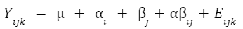
An example formula for a two-factor crossed ANOVA is:
How do I know which ANOVA to use?
As statisticians, we like to imagine that you’re reading this before you’ve run your experiment. You can save a lot of headache by simplifying an experiment into a standard format (when possible) to make the analysis straightforward.
Regardless, we’ll walk you through picking the right ANOVA for your experiment and provide examples for the most popular cases. The first question is:
Do you only have a single factor of interest?
If you have only measured a single factor (e.g., fertilizer A, fertilizer B, .etc.), then use one-way ANOVA . If you have more than one, then you need to consider the following:
Are you measuring the same observational unit (e.g., subject) multiple times?
This is where repeated measures come into play and can be a really confusing question for researchers, but if this sounds like it might describe your experiment, see repeated measures ANOVA . Otherwise:
Are any of the factors nested, where the levels are different depending on the levels of another factor?
In this case, you have a nested ANOVA design. If you don’t have nested factors or repeated measures, then it becomes simple:
Do you have two categorical factors?
Then use two-way ANOVA.
Do you have three categorical factors?
Use three-way ANOVA.
Do you have variables that you recorded that aren’t categorical (such as age, weight, etc.)?
Although these are outside the scope of this guide, if you have a single continuous variable, you might be able to use ANCOVA, which allows for a continuous covariate. With multiple continuous covariates, you probably want to use a mixed model or possibly multiple linear regression.
Prism does offer multiple linear regression but assumes that all factors are fixed. A full “mixed model” analysis is not yet available in Prism, but is offered as options within the one- and two-way ANOVA parameters.
How do I perform ANOVA?
Once you’ve determined which ANOVA is appropriate for your experiment, use statistical software to run the calculations. Below, we provide detailed examples of one, two and three-way ANOVA models.
How do I read and interpret an ANOVA table?
Interpreting any kind of ANOVA should start with the ANOVA table in the output. These tables are what give ANOVA its name, since they partition out the variance in the response into the various factors and interaction terms. This is done by calculating the sum of squares (SS) and mean squares (MS), which can be used to determine the variance in the response that is explained by each factor.
If you have predetermined your level of significance, interpretation mostly comes down to the p-values that come from the F-tests. The null hypothesis for each factor is that there is no significant difference between groups of that factor. All of the following factors are statistically significant with a very small p-value.
One-way ANOVA Example
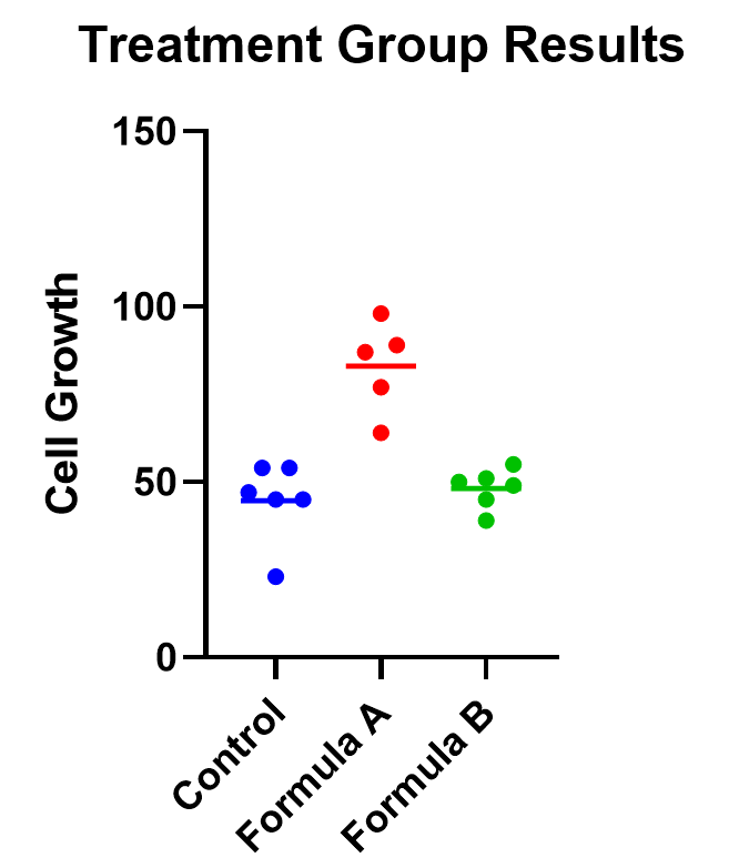
An example of one-way ANOVA is an experiment of cell growth in petri dishes. The response variable is a measure of their growth, and the variable of interest is treatment, which has three levels: formula A, formula B, and a control.
Classic one-way ANOVA assumes equal variances within each sample group. If that isn’t a valid assumption for your data, you have a number of alternatives .
Calculating a one-way ANOVA
Using Prism to do the analysis, we will run a one-way ANOVA and will choose 95% as our significance threshold. Since we are interested in the differences between each of the three groups, we will evaluate each and correct for multiple comparisons (more on this later!).
For the following, we’ll assume equal variances within the treatment groups. Consider
The first test to look at is the overall (or omnibus) F-test, with the null hypothesis that there is no significant difference between any of the treatment groups. In this case, there is a significant difference between the three groups (p<0.0001), which tells us that at least one of the groups has a statistically significant difference.
Now we can move to the heart of the issue, which is to determine which group means are statistically different. To learn more, we should graph the data and test the differences (using a multiple comparison correction).
Graphing one-way ANOVA
The easiest way to visualize the results from an ANOVA is to use a simple chart that shows all of the individual points. Rather than a bar chart, it’s best to use a plot that shows all of the data points (and means) for each group such as a scatter or violin plot.
As an example, below you can see a graph of the cell growth levels for each data point in each treatment group, along with a line to represent their mean. This can help give credence to any significant differences found, as well as show how closely groups overlap.
Determining statistical significance between groups
In addition to the graphic, what we really want to know is which treatment means are statistically different from each other. Because we are performing multiple tests, we’ll use a multiple comparison correction . For our example, we’ll use Tukey’s correction (although if we were only interested in the difference between each formula to the control, we could use Dunnett’s correction instead).
In this case, the mean cell growth for Formula A is significantly higher than the control (p<.0001) and Formula B ( p=0.002 ), but there’s no significant difference between Formula B and the control.

Two-way ANOVA example
For two-way ANOVA, there are two factors involved. Our example will focus on a case of cell lines. Suppose we have a 2x2 design (four total groupings). There are two different treatments (serum-starved and normal culture) and two different fields. There are 19 total cell line “experimental units” being evaluated, up to 5 in each group (note that with 4 groups and 19 observational units, this study isn’t balanced). Although there are multiple units in each group, they are all completely different replicates and therefore not repeated measures of the same unit.
As with one-way ANOVA, it’s a good idea to graph the data as well as look at the ANOVA table for results.
Graphing two-way ANOVA
There are many options here. Like our one-way example, we recommend a similar graphing approach that shows all the data points themselves along with the means.
Determining statistical significance between groups in two-way ANOVA
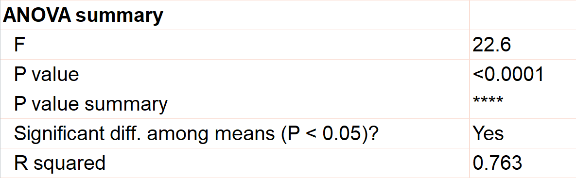
Let’s use a two-way ANOVA with a 95% significance threshold to evaluate both factors’ effects on the response, a measure of growth.
Feel free to use our two-way ANOVA checklist as often as you need for your own analysis.
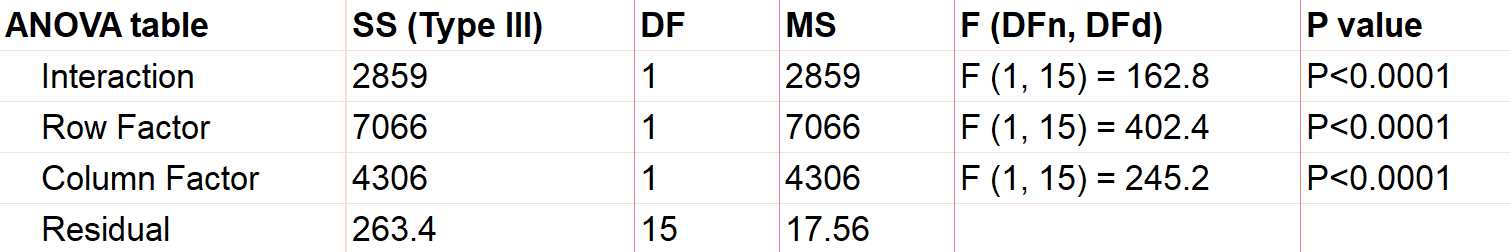
First, notice there are three sources of variation included in the model, which are interaction, treatment, and field.
The first effect to look at is the interaction term, because if it’s significant, it changes how you interpret the main effects (e.g., treatment and field). The interaction effect calculates if the effect of a factor depends on the other factor. In this case, the significant interaction term (p<.0001) indicates that the treatment effect depends on the field type.
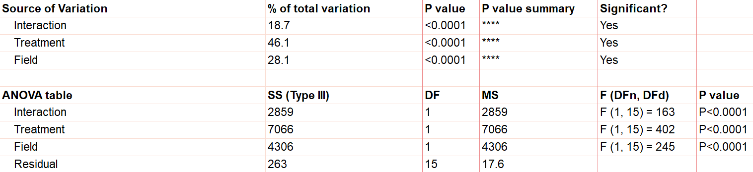
A significant interaction term muddies the interpretation, so that you no longer have the simple conclusion that “Treatment A outperforms Treatment B.” In this case, the graphic is particularly useful. It suggests that while there may be some difference between three of the groups, the precise combination of serum starved in field 2 outperformed the rest.
To confirm whether there is a statistically significant result, we would run pairwise comparisons (comparing each factor level combination with every other one) and account for multiple comparisons.
Do I need to correct for multiple comparisons for two-way ANOVA?
If you’re comparing the means for more than one combination of treatment groups, then absolutely! Here’s more information about multiple comparisons for two-way ANOVA .
Repeated measures ANOVA
So far we have focused almost exclusively on “ordinary” ANOVA and its differences depending on how many factors are involved. In all of these cases, each observation is completely unrelated to the others. Other than the combination of factors that may be the same across replicates, each replicate on its own is independent.
There is a second common branch of ANOVA known as repeated measures . In these cases, the units are related in that they are matched up in some way. Repeated measures are used to model correlation between measurements within an individual or subject. Repeated measures ANOVA is useful (and increases statistical power) when the variability within individuals is large relative to the variability among individuals.
It’s important that all levels of your repeated measures factor (usually time) are consistent. If they aren’t, you’ll need to consider running a mixed model, which is a more advanced statistical technique.
There are two common forms of repeated measures:
- You observe the same individual or subject at different time points. If you’re familiar with paired t-tests, this is an extension to that. (You can also have the same individual receive all of the treatments, which adds another level of repeated measures.)
- You have a randomized block design, where matched elements receive each treatment. For example, you split a large sample of blood taken from one person into 3 (or more) smaller samples, and each of those smaller samples gets exactly one treatment.
Repeated measures ANOVA can have any number of factors. See analysis checklists for one-way repeated measures ANOVA and two-way repeated measures ANOVA .
What does it mean to assume sphericity with repeated measures ANOVA?
Repeated measures are almost always treated as random factors, which means that the correlation structure between levels of the repeated measures needs to be defined. The assumption of sphericity means that you assume that each level of the repeated measures has the same correlation with every other level.
This is almost never the case with repeated measures over time (e.g., baseline, at treatment, 1 hour after treatment), and in those cases, we recommend not assuming sphericity. However, if you used a randomized block design, then sphericity is usually appropriate .
Example two-way ANOVA with repeated measures
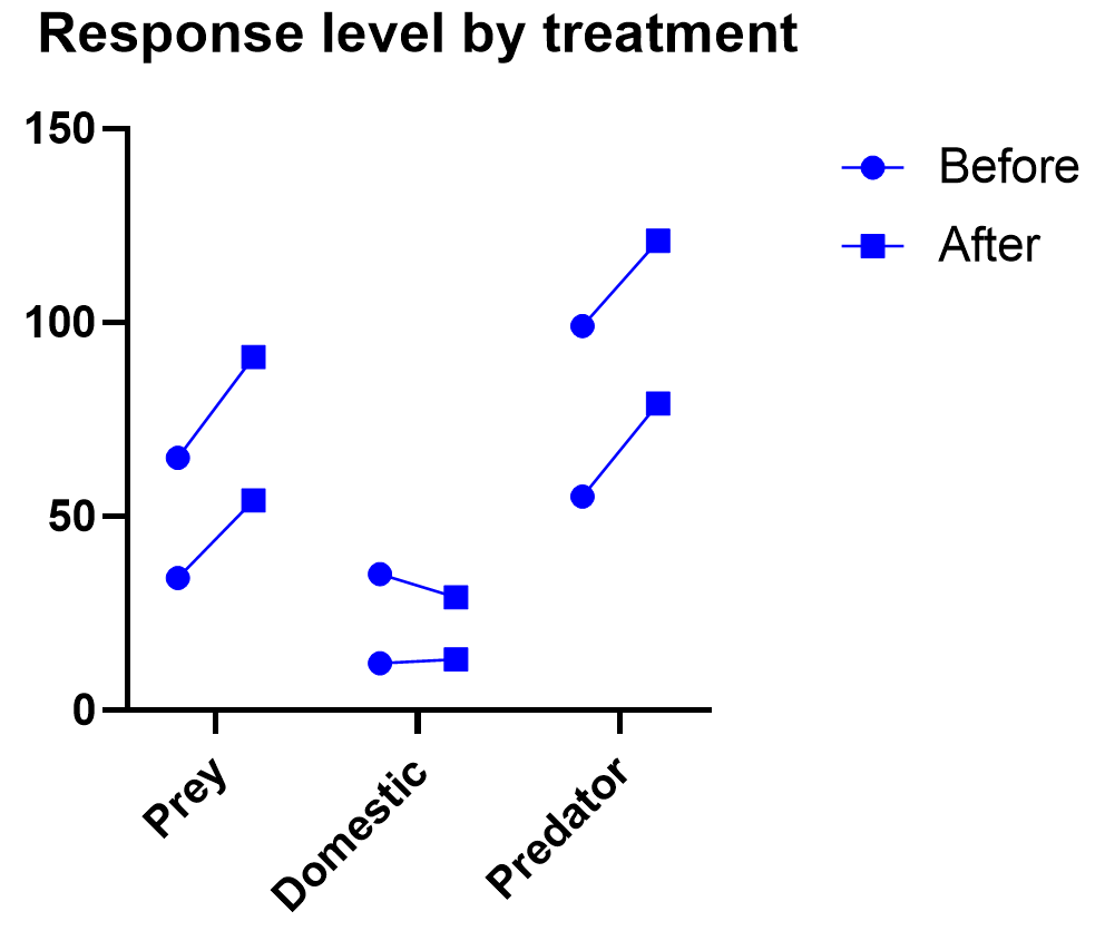
Say we have two treatments (control and treatment) to evaluate using test animals. We’ll apply both treatments to each two animals (replicates) with sufficient time in between the treatments so there isn’t a crossover (or carry-over) effect. Also, we’ll measure five different time points for each treatment (baseline, at time of injection, one hour after, …). This is repeated measures because we will need to measure matching samples from the same animal under each treatment as we track how its stimulation level changes over time.
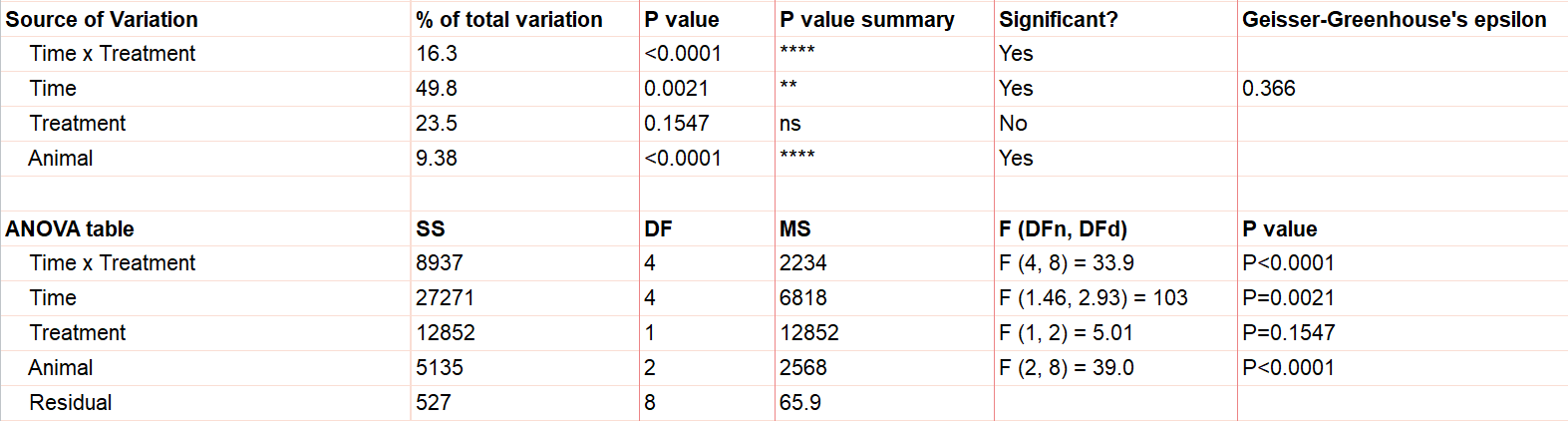
The output shows the test results from the main and interaction effects. Due to the interaction between time and treatment being significant (p<.0001), the fact that the treatment main effect isn’t significant (p=.154) isn’t noteworthy.
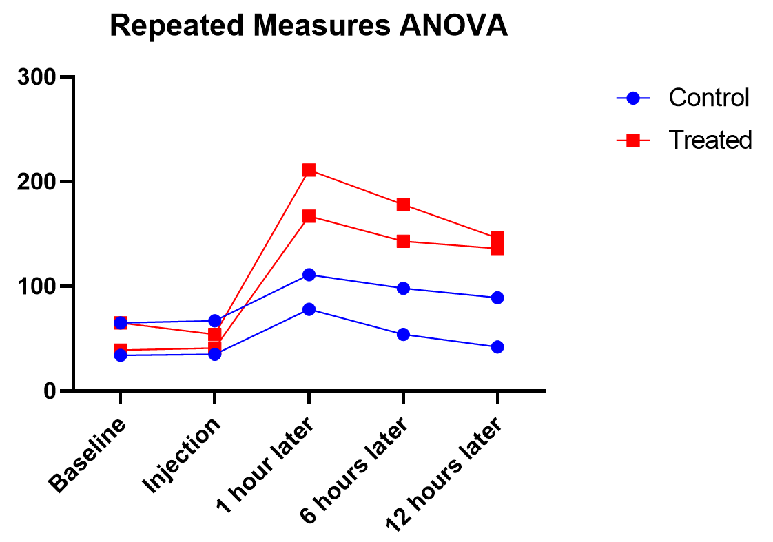
Graphing repeated measures ANOVA
As we’ve been saying, graphing the data is useful, and this is particularly true when the interaction term is significant. Here we get an explanation of why the interaction between treatment and time was significant, but treatment on its own was not. As soon as one hour after injection (and all time points after), treated units show a higher response level than the control even as it decreases over those 12 hours. Thus the effect of time depends on treatment. At the earlier time points, there is no difference between treatment and control.
Graphing repeated measures data is an art, but a good graphic helps you understand and communicate the results. For example, it’s a completely different experiment, but here’s a great plot of another repeated measures experiment with before and after values that are measured on three different animal types.
What if I have three or more factors?
Interpreting three or more factors is very challenging and usually requires advanced training and experience .
Just as two-way ANOVA is more complex than one-way, three-way ANOVA adds much more potential for confusion. Not only are you dealing with three different factors, you will now be testing seven hypotheses at the same time. Two-way interactions still exist here, and you may even run into a significant three-way interaction term.
It takes careful planning and advanced experimental design to be able to untangle the combinations that will be involved ( see more details here ).
Non-parametric ANOVA alternatives
As with t-tests (or virtually any statistical method), there are alternatives to ANOVA for testing differences between three groups. ANOVA is means-focused and evaluated in comparison to an F-distribution.
The two main non-parametric cousins to ANOVA are the Kruskal-Wallis and Friedman’s tests. Just as is true with everything else in ANOVA, it is likely that one of the two options is more appropriate for your experiment.
Kruskal-Wallis tests the difference between medians (rather than means) for 3 or more groups. It is only useful as an “ordinary ANOVA” alternative, without matched subjects like you have in repeated measures. Here are some tips for interpreting Kruskal-Wallis test results.
Friedman’s Test is the opposite, designed as an alternative to repeated measures ANOVA with matched subjects. Here are some tips for interpreting Friedman's Test .
What are simple, main, and interaction effects in ANOVA?
Consider the two-way ANOVA model setup that contains two different kinds of effects to evaluate:
The 𝛼 and 𝛽 factors are “main” effects, which are the isolated effect of a given factor. “Main effect” is used interchangeably with “simple effect” in some textbooks.
The interaction term is denoted as “𝛼𝛽”, and it allows for the effect of a factor to depend on the level of another factor. It can only be tested when you have replicates in your study. Otherwise, the error term is assumed to be the interaction term.
What are multiple comparisons?
When you’re doing multiple statistical tests on the same set of data, there’s a greater propensity to discover statistically significant differences that aren’t true differences. Multiple comparison corrections attempt to control for this, and in general control what is called the familywise error rate. There are a number of multiple comparison testing methods , which all have pros and cons depending on your particular experimental design and research questions.
What does the word “way” mean in one-way vs two-way ANOVA?
In statistics overall, it can be hard to keep track of factors, groups, and tails. To the untrained eye “two-way ANOVA” could mean any of these things.
The best way to think about ANOVA is in terms of factors or variables in your experiment. Suppose you have one factor in your analysis (perhaps “treatment”). You will likely see that written as a one-way ANOVA. Even if that factor has several different treatment groups, there is only one factor, and that’s what drives the name.
Also, “way” has absolutely nothing to do with “tails” like a t-test. ANOVA relies on F tests, which can only test for equal vs unequal because they rely on squared terms. So ANOVA does not have the “one-or-two tails” question .
What is the difference between ANOVA and a t-test?
ANOVA is an extension of the t-test. If you only have two group means to compare, use a t-test. Anything more requires ANOVA.
What is the difference between ANOVA and chi-square?
Chi-square is designed for contingency tables, or counts of items within groups (e.g., type of animal). The goal is to see whether the counts in a particular sample match the counts you would expect by random chance.
ANOVA separates subjects into groups for evaluation, but there is some numeric response variable of interest (e.g., glucose level).
Can ANOVA evaluate effects on multiple response variables at the same time?
Multiple response variables makes things much more complicated than multiple factors. ANOVA (as we’ve discussed it here) can obviously handle multiple factors but it isn’t designed for tracking more than one response at a time.
Technically, there is an expansion approach designed for this called Multivariate (or Multiple) ANOVA, or more commonly written as MANOVA. Things get complicated quickly, and in general requires advanced training.
Can ANOVA evaluate numeric factors in addition to the usual categorical factors?
It sounds like you are looking for ANCOVA (analysis of covariance). You can treat a continuous (numeric) factor as categorical, in which case you could use ANOVA, but this is a common point of confusion .
What is the definition of ANOVA?
ANOVA stands for analysis of variance, and, true to its name, it is a statistical technique that analyzes how experimental factors influence the variance in the response variable from an experiment.
What is blocking in Anova?
Blocking is an incredibly powerful and useful strategy in experimental design when you have a factor that you think will heavily influence the outcome, so you want to control for it in your experiment. Blocking affects how the randomization is done with the experiment. Usually blocking variables are nuisance variables that are important to control for but are not inherently of interest.
A simple example is an experiment evaluating the efficacy of a medical drug and blocking by age of the subject. To do blocking, you must first gather the ages of all of the participants in the study, appropriately bin them into groups (e.g., 10-30, 30-50, etc.), and then randomly assign an equal number of treatments to the subjects within each group.
There’s an entire field of study around blocking. Some examples include having multiple blocking variables, incomplete block designs where not all treatments appear in all blocks, and balanced (or unbalanced) blocking designs where equal (or unequal) numbers of replicates appear in each block and treatment combination.
What is ANOVA in statistics?
For a one-way ANOVA test, the overall ANOVA null hypothesis is that the mean responses are equal for all treatments. The ANOVA p-value comes from an F-test.
Can I do ANOVA in R?
While Prism makes ANOVA much more straightforward, you can use open-source coding languages like R as well. Here are some examples of R code for repeated measures ANOVA, both one-way ANOVA in R and two-way ANOVA in R .
Perform your own ANOVA
Are you ready for your own Analysis of variance? Prism makes choosing the correct ANOVA model simple and transparent .
Start your 30 day free trial of Prism and get access to:
- A step by step guide on how to perform ANOVA
- Sample data to save you time
- More tips on how Prism can help your research
With Prism, in a matter of minutes you learn how to go from entering data to performing statistical analyses and generating high-quality graphs.
- Skip to secondary menu
- Skip to main content
- Skip to primary sidebar
Statistics By Jim
Making statistics intuitive
ANOVA Overview
What is anova.
Analysis of variance (ANOVA) assesses the differences between group means. It is a statistical hypothesis test that determines whether the means of at least two populations are different. At a minimum, you need a continuous dependent variable and a categorical independent variable that divides your data into comparison groups to perform ANOVA.
Researchers commonly use ANOVA to analyze designed experiments. In these experiments, researchers use randomization and control the experimental factors in the treatment and control groups. For example, a product manufacturer sets the time and temperature settings in its process and records the product’s strength. ANOVA analyzes the differences in mean outcomes stemming from these experimental settings to estimate their effects and statistical significance. These designed experiments are typically orthogonal, which provides important benefits. Learn more about orthogonality .
Additionally, ANOVA is useful for observational studies . For example, a researcher can observe outcomes for several education methods and use ANOVA to analyze the group differences. However, as with any observational study, you must be careful about the conclusions you draw.
The term "analysis of variance" originates from how the analysis uses variances to determine whether the means are different. ANOVA works by comparing the variance of group means to the variance within groups. This process determines if the groups are part of one larger population or separate populations with different means. Consequently, even though it analyzes variances, it actually tests means! To learn more about this process, read my post, The F-test in ANOVA .
The fundamentals of ANOVA tests are relatively straightforward because it involves comparing means between groups. However, there are an array of elaborations. In this post, I start with the simpler forms and explain the essential jargon. Then I’ll broadly cover the more complex methods.
Simplest Form and Basic Terms of ANOVA Tests
The simplest type of ANOVA test is one-way ANOVA. This method is a generalization of t-tests that can assess the difference between more than two group means.

Statisticians consider ANOVA to be a special case of least squares regression, which is a specialization of the general linear model. All these models minimize the sum of the squared errors.
Related post : The Mean in Statistics
Factors and Factor Levels
To perform the most basic ANOVA, you need a continuous dependent variable and a categorical independent variable. In ANOVA lingo, analysts refer to “categorical independent variables” as factors. The categorical values of a factor are “levels.” These factor levels create the groups in the data. Factor level means are the means of the dependent variable associated with each factor level.
For example, your factor might have the following three levels in an experiment: Control, Treatment 1, and Treatment 2. The ANOVA test will determine whether the mean outcomes for these three conditions (i.e., factor levels) are different.
Related posts : Independent and Dependent Variables and Control Groups in Experiments
Factor Level Combinations
ANOVA allows you to include more than one factor. For example, you might want to determine whether gender and college major correspond to differences in income.
Gender is one factor with two levels: Male and Female. College major is another factor with three levels in our fictional study: Statistics, Psychology, and Political Science.
The combination of these two factors (2 genders X 3 majors) creates the following six groups:
- Male / Statistics
- Female / Statistics
- Male / Psychology
- Female Psychology
- Male / Political Science
- Female / Political Science
These groups are the factor level combinations. ANOVA determines whether the mean incomes for these groups are different.
Factorial ANOVA
ANOVA allows you to assess multiple factors simultaneously. Factorial ANOVA are cases where your data includes observations for all the factor level combinations that your model specifies. For example, using the gender and college major model, you are performing factorial ANOVA if your dataset includes income observations for all six groups.
By assessing multiple factors together, factorial ANOVA allows your model to detect interaction effects. This ability makes multiple factor ANOVA much more efficient. Additionally, evaluating a single factor at a time conceals interaction effects. Single-factor analyses tend to produce inconsistent results when interaction effects exist in an experimental area because they cannot model the interaction effects.
Analysts frequently use factorial ANOVA in experiments because they efficiently test the main and interaction effects for all experimental factors.
Related post : Understanding Interaction Effects
Interpreting the ANOVA Test
ANOVA assesses differences between group means.
Suppose you compare two new teaching methods to the standard practice and want to know if the average test scores for the methods are different. Your factor is Teaching Method, and it contains the following three levels: Standard, Method A, and Method B.
The factor level means are the mean test score associated with each group.
ANOVAs evaluate the differences between the means of the dependent variable for the factor level combinations. The hypotheses for the ANOVA test are the following:
- Null Hypothesis: The group means are all equal.
- Alternative Hypothesis: At least one mean is different.
When the p-value is below your significance level, reject the null hypothesis. Your data favor the position that at least one group mean is different from the others.
While a significant ANOVA result indicates that at least one mean differs, it does not specify which one. To identify which differences between pairs of means are statistically significant, you’ll need to perform a post hoc analysis .
Related post : How to Interpret P Values
General ANOVA Assumptions
ANOVA tests have the same assumptions as other linear models other than requiring a factor. Specifically:
- The dependent variable is continuous.
- You have at least one categorical independent variable (factor).
- The observations are independent.
- The groups should have roughly equal variances (scatter).
- The data in the groups should follow a normal distribution.
- The residuals satisfy the ordinary least squares assumptions .
While ANOVA assumes your data follow the normal distribution, it is robust to violations of this assumption when your groups have at least 15 observations.
ANOVA Designs and Types of Models
The simpler types of ANOVA test are relatively straightforward. However, ANOVA is a flexible analysis, and many elaborations are possible. I’ll start with the simple forms and move to the more complex designs. Click the links to learn more about each type and see examples of them in action!
One-way ANOVA
One-way ANOVA tests one factor that divides the data into at least two independent groups.
Learn about one-way ANOVA and how to perform and interpret an example using Excel.
Two-way ANOVA
Two-way ANOVA tests include two factors that divide the data into at least four factor level combinations. In addition to identifying the factors’ main effects, these models evaluate interaction effects between the factors.
Learn about two-way ANOVA and how to perform and interpret an example using Excel.
Analysis of Covariance (ANCOVA)
ANCOVA models include factors and covariates. Covariates are continuous independent variables that have a relationship with the dependent variable. Typically, covariates are nuisance variables that researchers cannot control during an experiment. Consequently, analysts include covariates in the model to control them statistically.
Learn more about Covariates: Definition and Uses .
Repeated measures ANOVA
Repeated measures designs allow researchers to assess participants multiple times in a study. Frequently, the subjects serve as their own controls and experience several treatment conditions.
Learn about repeated measures ANOVA tests and see an example.
Multivariate analysis of variance (MANOVA)
MANOVA extends the capabilities of ANOVA by assessing multiple dependent variables simultaneously. The factors in MANOVA can influence the relationship between dependent variables instead of influencing a single dependent variable.
There’s even a MANCOVA, which is MANOVA plus ANCOVA! It allows you to include covariates when modeling multiple independent variables.
Learn about MANOVA and see an example.
Crossed and Nested Models
ANOVA can model both crossed and nested factors.
Crossed factors are the more familiar type. Two factors are crossed when each level of a factor occurs with each level of the other factor. The gender and college major factors in the earlier example are crossed because we have all combinations of the factor levels. All levels of gender occur in all majors and vice versa.
A factor is nested in another factor when all its levels occur within only one level of the other factor. Consequently, the data do not contain all possible factor level combinations. For example, suppose you are testing bug spray effectiveness, and your factors are Brand and Product.

In the illustration, Product is nested within Brand because each product occurs within only one level of Brand. There can be no combination that represents Brand 2 and Product A.
The combinations of crossed and nested factors within an ANOVA design can become quite complex!
General Linear Model
The most general form of ANOVA allows you to include all the above and more! In your model, you can have as many factors and covariates as you need, interaction terms, crossed and nested factors, along with specifying fixed, random, or mixed effects, which I describe below.
Types of Effects in ANOVA
Fixed effects.
When a researcher can set the factor levels in an experiment, it is a fixed factor. Correspondingly, the model estimates fixed effects for fixed factors. Fixed effects are probably the type with which you’re most familiar. One-way and two-way ANOVA procedures typically use fixed-effects models. ANOVA models usually assess fixed using ordinary least squares.
For example, in a cake recipe experiment, the researcher sets the three oven temperatures of 350, 400, and 450 degrees for the study. Oven temperature is a fixed factor.
Random effects
When a researcher samples the factor levels from a population rather than setting them, it is a random factor. The model estimates random effects for them. Because random factors sample data from a population, the model must change how it evaluates their effects by calculating variance components .
For example, in studies involving human subjects, Subject is typically a random factor because researchers sample participants from a population.
Mixed effects
Mixed-effects models contain both fixed and random effects. Frequently, mixed-effects models use restricted maximum likelihood (REML) to estimate effects.
For example, a store chain wants to assess sales. The chain chooses five states for its study. State is a fixed factor. Within these states, the chain randomly selects stores. Store is a random factor. It is also nested within the State factor.
Scroll down to find more of my articles about ANOVA!
One Way ANOVA Overview & Example
By Jim Frost Leave a Comment
What is One Way ANOVA?
Use one way ANOVA to compare the means of three or more groups. This analysis is an inferential hypothesis test that uses samples to draw conclusions about populations. Specifically, it tells you whether your sample provides sufficient evidence to conclude that the groups’ population means are different. ANOVA stands for analysis of variance. [Read more…] about One Way ANOVA Overview & Example
ANCOVA: Uses, Assumptions & Example
By Jim Frost 1 Comment
What is ANCOVA?
ANCOVA, or the analysis of covariance, is a powerful statistical method that analyzes the differences between three or more group means while controlling for the effects of at least one continuous covariate. [Read more…] about ANCOVA: Uses, Assumptions & Example
Covariates: Definition & Uses
By Jim Frost 9 Comments
What is a Covariate?
Covariates are continuous independent variables (or predictors) in a regression or ANOVA model. These variables can explain some of the variability in the dependent variable.
That definition of covariates is simple enough. However, the usage of the term has changed over time. Consequently, analysts can have drastically different contexts in mind when discussing covariates. [Read more…] about Covariates: Definition & Uses
How to do Two-Way ANOVA in Excel
By Jim Frost 35 Comments
Use two-way ANOVA to assess differences between the group means that are defined by two categorical factors . In this post, we’ll work through two-way ANOVA using Excel. Even if Excel isn’t your main statistical package, this post is an excellent introduction to two-way ANOVA. Excel refers to this analysis as two factor ANOVA. [Read more…] about How to do Two-Way ANOVA in Excel
How to do One-Way ANOVA in Excel
By Jim Frost 23 Comments
Use one-way ANOVA to test whether the means of at least three groups are different. Excel refers to this test as Single Factor ANOVA. This post is an excellent introduction to performing and interpreting a one-way ANOVA test even if Excel isn’t your primary statistical software package. [Read more…] about How to do One-Way ANOVA in Excel
Using Post Hoc Tests with ANOVA
By Jim Frost 138 Comments
Post hoc tests are an integral part of ANOVA. When you use ANOVA to test the equality of at least three group means, statistically significant results indicate that not all of the group means are equal. However, ANOVA results do not identify which particular differences between pairs of means are significant. Use post hoc tests to explore differences between multiple group means while controlling the experiment-wise error rate.
In this post, I’ll show you what post hoc analyses are, the critical benefits they provide, and help you choose the correct one for your study. Additionally, I’ll show why failure to control the experiment-wise error rate will cause you to have severe doubts about your results. [Read more…] about Using Post Hoc Tests with ANOVA
How F-tests work in Analysis of Variance (ANOVA)
By Jim Frost 51 Comments
Analysis of variance (ANOVA) uses F-tests to statistically assess the equality of means when you have three or more groups. In this post, I’ll answer several common questions about the F-test.
- How do F-tests work?
- Why do we analyze variances to test means ?
I’ll use concepts and graphs to answer these questions about F-tests in the context of a one-way ANOVA example. I’ll use the same approach that I use to explain how t-tests work . If you need a primer on the basics, read my hypothesis testing overview .
To learn more about ANOVA tests, including the more complex forms, read my ANOVA Overview and One-Way ANOVA Overview and Example .
[Read more…] about How F-tests work in Analysis of Variance (ANOVA)
Benefits of Welch’s ANOVA Compared to the Classic One-Way ANOVA
By Jim Frost 70 Comments
Welch’s ANOVA is an alternative to the traditional analysis of variance (ANOVA) and it offers some serious benefits. One-way analysis of variance determines whether differences between the means of at least three groups are statistically significant. For decades, introductory statistics classes have taught the classic Fishers one-way ANOVA that uses the F-test. It’s a standard statistical analysis, and you might think it’s pretty much set in stone by now. Surprise, there’s a significant change occurring in the world of one-way analysis of variance! [Read more…] about Benefits of Welch’s ANOVA Compared to the Classic One-Way ANOVA
Multivariate ANOVA (MANOVA) Benefits and When to Use It
By Jim Frost 181 Comments
Multivariate ANOVA (MANOVA) extends the capabilities of analysis of variance (ANOVA) by assessing multiple dependent variables simultaneously. ANOVA statistically tests the differences between three or more group means. For example, if you have three different teaching methods and you want to evaluate the average scores for these groups, you can use ANOVA. However, ANOVA does have a drawback. It can assess only one dependent variable at a time. This limitation can be an enormous problem in certain circumstances because it can prevent you from detecting effects that actually exist. [Read more…] about Multivariate ANOVA (MANOVA) Benefits and When to Use It
Repeated Measures Designs: Benefits and an ANOVA Example
By Jim Frost 25 Comments
Repeated measures designs, also known as a within-subjects designs, can seem like oddball experiments. When you think of a typical experiment, you probably picture an experimental design that uses mutually exclusive, independent groups. These experiments have a control group and treatment groups that have clear divisions between them. Each subject is in only one of these groups. [Read more…] about Repeated Measures Designs: Benefits and an ANOVA Example
ANOVA (Analysis of Variance)
ANOVA, short for Analysis of Variance, is a statistical method used to see if there are significant differences between the averages of three or more unrelated groups. This technique is especially useful when comparing more than two groups, which is a limitation of other tests like the t-test and z-test. For example, ANOVA can compare average IQ scores across several countries—like the US, Canada, Italy, and Spain—to see if nationality influences IQ scores. Ronald Fisher developed ANOVA in 1918, expanding the capabilities of previous tests by allowing for the comparison of multiple groups at once. This method is also referred to as Fisher’s analysis of variance, highlighting its ability to analyze how a categorical variable with multiple levels affects a continuous variable.
The use of ANOVA depends on the research design. Commonly, ANOVAs are used in three ways: one-way ANOVA , two-way ANOVA , and N-way ANOVA.
One-Way ANOVA
One-Way ANOVA is a statistical method used when we’re looking at the impact of one single factor on a particular outcome. For instance, if we want to explore how IQ scores vary by country, that’s where One-Way ANOVA comes into play. The “one way” part means we’re only considering one independent variable, which in this case is the country, but remember, this country variable can include any number of categories, from just two countries to twenty or more.
Two-Way ANOVA
Moving a step further, Two-Way ANOVA, also known as factorial ANOVA, allows us to examine the effect of two different factors on an outcome simultaneously. Building on our previous example, we could look at how both country and gender influence IQ scores. This method doesn’t just tell us about the individual effects of each factor but also lets us explore interactions between them. An interaction effect means the impact of one factor might change depending on the level of the other factor. For example, the difference in IQ scores between genders might vary from one country to another, suggesting that the effect of gender on IQ is not consistent across all countries.
N-Way ANOVA
When researchers have more than two factors to consider, they turn to N-Way ANOVA, where “n” represents the number of independent variables in the analysis. This could mean examining how IQ scores are influenced by a combination of factors like country, gender, age group, and ethnicity all at once. N-Way ANOVA allows for a comprehensive analysis of how these multiple factors interact with each other and their combined effect on the dependent variable, providing a deeper understanding of the dynamics at play.
In summary, ANOVA is a versatile statistical tool that scales from analyzing the effect of one factor (One-Way ANOVA) to multiple factors (Two-Way or N-Way ANOVA) on an outcome. By using ANOVA, researchers can uncover not just the direct effects of independent variables on a dependent variable but also how these variables interact with each other, offering rich insights into complex phenomena.
Looking for assistance with your research?
Schedule a time to speak with an expert using the calendar below.
User-friendly Software
Transform raw data to written interpreted results in seconds.
General Purpose and Procedure
Omnibus ANOVA test:
The null hypothesis for an ANOVA is that there is no significant difference among the groups. The alternative hypothesis assumes that there is at least one significant difference among the groups. After cleaning the data, the researcher must test the assumptions of ANOVA. They must then calculate the F -ratio and the associated probability value ( p -value). In general, if the p -value associated with the F is smaller than .05, then the null hypothesis is rejected and the alternative hypothesis is supported. If the null hypothesis is rejected, one concludes that the means of all the groups are not equal. Post-hoc tests tell the researcher which groups are different from each other.
So what if you find statistical significance? Multiple comparison tests
When you conduct an ANOVA, you are attempting to determine if there is a statistically significant difference among the groups. If you find that there is a difference, you will then need to examine where the group differences lay.
At this point you could run post-hoc tests which are t tests examining mean differences between the groups. There are several multiple comparison tests that can be conducted that will control for Type I error rate, including the Bonferroni , Scheffe, Dunnet, and Tukey tests.
Research Questions the ANOVA Examines
One-way ANOVA: Are there differences in GPA by grade level (freshmen vs. sophomores vs. juniors)?
Two-way ANOVA: Are there differences in GPA by grade level (freshmen vs. sophomores vs. juniors) and gender (male vs. female)?
Data Level and Assumptions
The level of measurement of the variables and assumptions of the test play an important role in ANOVA. In ANOVA, the dependent variable must be a continuous (interval or ratio) level of measurement. The independent variables in ANOVA must be categorical (nominal or ordinal) variables. Like the t -test, ANOVA is also a parametric test and has some assumptions. ANOVA assumes that the data is normally distributed. The ANOVA also assumes homogeneity of variance, which means that the variance among the groups should be approximately equal. ANOVA also assumes that the observations are independent of each other. Researchers should keep in mind when planning any study to look out for extraneous or confounding variables. ANOVA has methods (i.e., ANCOVA) to control for confounding variables.
Testing of the Assumptions
- The population from which samples are drawn should be normally distributed.
- Independence of cases: the sample cases should be independent of each other.
- Homogeneity of variance: Homogeneity means that the variance among the groups should be approximately equal.
These assumptions can be tested using statistical software (like Intellectus Statistics!). The assumption of homogeneity of variance can be tested using tests such as Levene’s test or the Brown-Forsythe Test. Normality of the distribution of the scores can be tested using histograms, the values of skewness and kurtosis, or using tests such as Shapiro-Wilk or Kolmogorov-Smirnov. The assumption of independence can be determined from the design of the study.
It is important to note that ANOVA is not robust to violations to the assumption of independence. This is to say, that even if you violate the assumptions of homogeneity or normality, you can conduct the test and basically trust the findings. However, the results of the ANOVA are invalid if the independence assumption is violated. In general, with violations of homogeneity the analysis is considered robust if you have equal sized groups. With violations of normality, continuing with the ANOVA is generally ok if you have a large sample size .
Related Analyses: MANOVA and ANCOVA
Researchers have extended ANOVA in MANOVA and ANCOVA. MANOVA stands for the multivariate analysis of variance. MANOVA is used when there are two or more dependent variables. ANCOVA is the term for analysis of covariance. The ANCOVA is used when the researcher includes one or more covariate variables in the analysis.
Need more help?
Check out our online course for conducting an ANOVA here .
Algina, J., & Olejnik, S. (2003). Conducting power analyses for ANOVA and ANCOVA in between-subjects designs. Evaluation & the Health Professions, 26 (3), 288-314.
Cardinal, R. N., & Aitken, M. R. F. (2006). ANOVA for the behavioural sciences researcher . Mahwah, NJ: Lawrence Erlbaum Associates.
Davison, M. L., & Sharma, A. R. (1994). ANOVA and ANCOVA of pre- and post-test, ordinal data. Psychometrika, 59 (4), 593-600.
Levy, M. S., & Neill, J. W. (1990). Testing for lack of fit in linear multiresponse models based on exact or near replicates. Communications in Statistics – Theory and Methods, 19 (6), 1987-2002.
Tsangari, H., & Akritas, M. G. (2004). Nonparametric ANCOVA with two and three covariates. Journal of Multivariate Analysis, 88 (2), 298-319.
Turner, J. R., & Thayer, J. F. (2001). Introduction to analysis of variance: Design, analysis, & interpretation . Thousand Oaks, CA: Sage Publications.
Wilcox, R. R. (2005). An approach to ANCOVA that allows multiple covariates, nonlinearity, and heteroscedasticity. Educational and Psychological Measurement, 65 (3), 442-450.
Wright, D. B. (2006). Comparing groups in a before-after design: When t test and ANCOVA produce different results. British Journal of Educational Psychology, 76 , 663-675.
To Reference this Page : Statistics Solutions. (2013). ANOVA . Retrieved from https://www.statisticssolutions.com/free-resources/directory-of-statistical-analyses/anova/
Related Pages:
- Conduct and Interpret a One-Way ANOVA
- Conduct and Interpret a Factorial ANOVA
- Conduct and Interpret a Repeated Measures ANOVA
Statistics Solutions can assist with your quantitative analysis by assisting you to develop your methodology and results chapters. The services that we offer include:
Data Analysis Plan
- Edit your research questions and null/alternative hypotheses
- Write your data analysis plan; specify specific statistics to address the research questions, the assumptions of the statistics, and justify why they are the appropriate statistics; provide references
- Justify your sample size/power analysis, provide references
- Explain your data analysis plan to you so you are comfortable and confident
- Two hours of additional support with your statistician
Quantitative Results Section (Descriptive Statistics, Bivariate and Multivariate Analyses, Structural Equation Modeling , Path analysis, HLM, Cluster Analysis )
- Clean and code dataset
- Conduct descriptive statistics (i.e., mean, standard deviation, frequency and percent, as appropriate)
- Conduct analyses to examine each of your research questions
- Write-up results
- Provide APA 7 th edition tables and figures
- Explain Chapter 4 findings
- Ongoing support for entire results chapter statistics
Please call 727-442-4290 to request a quote based on the specifics of your research, schedule using the calendar on this page, or email [email protected]

An official website of the United States government
The .gov means it’s official. Federal government websites often end in .gov or .mil. Before sharing sensitive information, make sure you’re on a federal government site.
The site is secure. The https:// ensures that you are connecting to the official website and that any information you provide is encrypted and transmitted securely.
- Publications
- Account settings
Preview improvements coming to the PMC website in October 2024. Learn More or Try it out now .
- Advanced Search
- Journal List
- Korean J Anesthesiol
- v.70(1); 2017 Feb
Understanding one-way ANOVA using conceptual figures
Tae kyun kim.
Department of Anesthesia and Pain Medicine, Pusan National University Yangsan Hospital and School of Medicine, Yangsan, Korea.
Analysis of variance (ANOVA) is one of the most frequently used statistical methods in medical research. The need for ANOVA arises from the error of alpha level inflation, which increases Type 1 error probability (false positive) and is caused by multiple comparisons. ANOVA uses the statistic F, which is the ratio of between and within group variances. The main interest of analysis is focused on the differences of group means; however, ANOVA focuses on the difference of variances. The illustrated figures would serve as a suitable guide to understand how ANOVA determines the mean difference problems by using between and within group variance differences.
Introduction
The differences in the means of two groups that are mutually independent and satisfy both the normality and equal variance assumptions can be obtained by comparing them using a Student's t-test. However, we may have to determine whether differences exist in the means of 3 or more groups. Most readers are already aware of the fact that the most common analytical method for this is the one-way analysis of variance (ANOVA). The present article aims to examine the necessity of using a one-way ANOVA instead of simply repeating the comparisons using Student's t-test. ANOVA literally means analysis of variance, and the present article aims to use a conceptual illustration to explain how the difference in means can be explained by comparing the variances rather by the means themselves.
Significance Level Inflation
In the comparison of the means of three groups that are mutually independent and satisfy the normality and equal variance assumptions, when each group is paired with another to attempt three paired comparisons 1) , the increase in Type I error becomes a common occurrence. In other words, even though the null hypothesis is true, the probability of rejecting it increases, whereby the probability of concluding that the alternative hypothesis (research hypothesis) has significance increases, despite the fact that it has no significance.
Let us assume that the distribution of differences in the means of two groups is as shown in Fig. 1 . The maximum allowable error range that can claim “differences in means exist” can be defined as the significance level (α). This is the maximum probability of Type I error that can reject the null hypothesis of “differences in means do not exist” in the comparison between two mutually independent groups obtained from one experiment. When the null hypothesis is true, the probability of accepting it becomes 1-α.

Now, let us compare the means of three groups. Often, the null hypothesis in the comparison of three groups would be “the population means of three groups are all the same,” however, the alternative hypothesis is not “the population means of three groups are all different,” but rather, it is “at least one of the population means of three groups is different.” In other words, the null hypothesis (H 0 ) and the alternative hypothesis (H 1 ) are as follows:
Therefore, among the three groups, if the means of any two groups are different from each other, the null hypothesis can be rejected.
In that case, let us examine whether the probability of rejecting the entire null hypothesis remains consistent, when two continuous comparisons are made on hypotheses that are not mutually independent. When the null hypothesis is true, if the null hypothesis is rejected from a single comparison, then the entire null hypothesis can be rejected. Accordingly, the probability of rejecting the entire null hypothesis from two comparisons can be derived by firstly calculating the probability of accepting the null hypothesis from two comparisons, and then subtracting that value from 1. Therefore, the probability of rejecting the entire null hypothesis from two comparisons is as follows:
If the comparisons are made n times, the probability of rejecting the entire null hypothesis can be expressed as follows:
It can be seen that as the number of comparisons increases, the probability of rejecting the entire null hypothesis also increases. Assuming the significance level for a single comparison to be 0.05, the increases in the probability of rejecting the entire null hypothesis according to the number of comparisons are shown in Table 1 .
| Number of comparisons | Significance level |
|---|---|
| 1 | 0.05 |
| 2 | 0.098 |
| 3 | 0.143 |
| 4 | 0.185 |
| 5 | 0.226 |
| 6 | 0.265 |
ANOVA Table
Although various methods have been used to avoid the hypothesis testing error due to significance level inflation, such as adjusting the significance level by the number of comparisons, the ideal method for resolving this problem as a single statistic is the use of ANOVA. ANOVA is an acronym for analysis of variance, and as the name itself implies, it is variance analysis. Let us examine the reason why the differences in means can be explained by analyzing the variances, despite the fact that the core of the problem that we want to figure out lies with the comparisons of means.
For example, let us examine whether there are differences in the height of students according to their grades ( Table 2 ). First, let us examine the ANOVA table ( Table 3 ) that is commonly obtained as a product of ANOVA. In Table 3 , the significance is ultimately determined using a significance probability value (P value), and in order to obtain this value, the statistic and its position in the distribution to which it belongs, must be known. In other words, there has to be a distribution that serves as the reference and that distribution is called F distribution. This F comes from the name of the statistician Ronald Fisher . The ANOVA test is also referred to as the F test, and F distribution is a distribution formed by the variance ratios. Accordingly, F statistic is expressed as a variance ratio, as shown below.
| Class A (n = 30) | Class B (n = 30) | Class C (n = 30) | |||
|---|---|---|---|---|---|
| 156 | 171.2 | 156.6 | 169.3 | 156.7 | 173.5 |
| 160.4 | 171.3 | 160.1 | 169.4 | 161.9 | 173.6 |
| 161.7 | 171.5 | 161 | 169.5 | 162.9 | 173.9 |
| 163.6 | 171.9 | 161.2 | 170.7 | 165 | 174.2 |
| 163.8 | 172 | 161.4 | 170.7 | 165.5 | 175.4 |
| 164.8 | 172 | 162.5 | 172.2 | 166.1 | 175.6 |
| 165.8 | 172.9 | 162.6 | 172.9 | 166.2 | 176.4 |
| 165.8 | 173.5 | 162.9 | 173.9 | 166.2 | 177.7 |
| 166.2 | 173.8 | 163.1 | 173.9 | 167.1 | 179.3 |
| 168 | 173.9 | 164.4 | 174.1 | 169.1 | 179.8 |
| 168.1 | 174 | 165.9 | 174.3 | 170.9 | 180 |
| 168.4 | 175.7 | 166 | 174.9 | 171.4 | 180.3 |
| 168.7 | 175.8 | 166.3 | 175.4 | 172 | 181.6 |
| 169.4 | 176.7 | 167.3 | 176.7 | 172.2 | 182.1 |
| 170 | 187 | 168.9 | 178.7 | 173.3 | 183.7 |
Raw data of students' heights in three different classes. Each class consists of thirty students.
| Sum of squares | Freedom | Mean sum of squares | F | Significance probability | |
|---|---|---|---|---|---|
| Intergroup | 273.875 | 2 | 136.937 | 3.629 | 0.031 |
| ( − 1) | |||||
| Intragroup | 3282.843 | 87 | 37.734 | ||
| ( − ) | |||||
| Overall | 3556.718 | 89 |
Ȳ i is the mean of the group i; n i is the number of observations of the group i; Ȳ is the overall mean; K is the number of groups; Y ij is the j th observational value of group i; and N is the number of all observational values. The F statistic is the ratio of intergroup mean sum of squares to intragroup mean sum of squares.
Here, Ȳ i is the mean of the group i; n i is the number of observations of the group i; Ȳ is the overall mean; K is the number of groups; Y ij is the j th observational value of group i; and N is the number of all observational values.
It is not easy to look at this complex equation and understand ANOVA at a single glance. The meaning of this equation will be explained as an illustration for easier understanding. Statistics can be regarded as a study field that attempts to express data which are difficult to understand with an easy and simple ways so that they can be represented in a brief and simple forms. What that means is, instead of independently observing the groups of scattered points, as shown in Fig. 2A , the explanation could be given with the points lumped together as a single representative value. Values that are commonly referred to as the mean, median, and mode can be used as the representative value. Here, let us assume that the black rectangle in the middle represents the overall mean. However, a closer look shows that the points inside the circle have different shapes and the points with the same shape appear to be gathered together. Therefore, explaining all the points with just the overall mean would be inappropriate, and the points would be divided into groups in such a way that the same shapes belong to the same group. Although it is more cumbersome than explaining the entire population with just the overall mean, it is more reasonable to first form groups of points with the same shape and establish the mean for each group, and then explain the population with the three means. Therefore, as shown in Fig. 2B , the groups were divided into three and the mean was established in the center of each group in an effort to explain the entire population with these three points. Now the question arises as to how can one evaluate whether there are differences in explaining with the representative value of the three groups (e.g.; mean) versus explaining with lumping them together as a single overall mean.

First, let us measure the distance between the overall mean and the mean of each group, and the distance from the mean of each group to each data within that group. The distance between the overall mean and the mean of each group was expressed as a solid arrow line ( Fig. 2C ). This distance is expressed as (Ȳ i − Ȳ) 2 , which appears in the denominator of the equation for calculating the F statistic. Here, the number of data in each group are multiplied, n i (Ȳ i − Ȳ) 2 . This is because explaining with the representative value of a single group is the same as considering that all the data in that group are accumulated at the representative value. Therefore, the amount of variance which is induced by explaining with the points divided into groups can be seen, as compared to explaining with the overall mean, and this explains inter-group variance.
Let us return to the equation for deriving the F statistic. The meaning of ( Y ij − Ȳ i ) 2 in the numerator is represented as an illustration in Fig. 2C , and the distance from the mean of each group to each data is shown by the dotted line arrows. In the figure, this distance represents the distance from the mean within the group to the data within that group, which explains the intragroup variance.
By looking at the equation for F statistic, it can be seen that this inter- or intragroup variance was divided into inter- and intragroup freedom. Let us assume that when all the fingers are stretched out, the mean value of the finger length is represented by the index finger. If the differences in finger lengths are compared to find the variance, then it can be seen that although there are 5 fingers, the number of gaps between the fingers is 4. To derive the mean variance, the intergroup variance was divided by freedom of 2, while the intragroup variance was divided by the freedom of 87, which was the overall number obtained by subtracting 1 from each group.
What can be understood by deriving the variance can be described in this manner. In Figs. 3A and 3B , the explanations are given with two different examples. Although the data were divided into three groups, there may be cases in which the intragroup variance is too big ( Fig. 3A ), so it appears that nothing is gained by dividing into three groups, since the boundaries become ambiguous and the group mean is not far from the overall mean. It seems that it would have been more efficient to explain the entire population with the overall mean. Alternatively, when the intergroup variance is relatively larger than the intragroup variance, in other word, when the distance from the overall mean to the mean of each group is far ( Fig. 3B ), the boundaries between the groups become more clear, and explaining by dividing into three group appears more logical than lumping together as the overall mean.

Ultimately, the positions of statistic derived in this manner from the inter- and intragroup variance ratios can be identified from the F distribution ( Fig. 4 ). When the statistic 3.629 in the ANOVA table is positioned more to the right than 3.101, which is a value corresponding to the significance level of 0.05 in the F distribution with freedoms of 2 and 87, meaning bigger than 3.101, the null hypothesis can be rejected.

Post-hoc Test
Anyone who has performed ANOVA has heard of the term post-hoc test. It refers to “the analysis after the fact” and it is derived from the Latin word for “after that.” The reason for performing a post-hoc test is that the conclusions that can be derived from the ANOVA test have limitations. In other words, when the null hypothesis that says the population means of three mutually independent groups are the same is rejected, the information that can be obtained is not that the three groups are different from each other. It only provides information that the means of the three groups may differ and at least one group may show a difference. This means that it does not provide information on which group differs from which other group ( Fig. 5 ). As a result, the comparisons are made with different pairings of groups, undergoing an additional process of verifying which group differs from which other group. This process is referred to as the post-hoc test.

The significance level is adjusted by various methods [ 1 ], such as dividing the significance level by the number of comparisons made. Depending on the adjustment method, various post-hoc tests can be conducted. Whichever method is used, there would be no major problems, as long as that method is clearly described. One of the most well-known methods is the Bonferroni's correction. To explain this briefly, the significance level is divided by the number of comparisons and applied to the comparisons of each group. For example, when comparing the population means of three mutually independent groups A, B, and C, if the significance level is 0.05, then the significance level used for comparisons of groups A and B, groups A and C, and groups B and C would be 0.05/3 = 0.017. Other methods include Turkey, Schéffe, and Holm methods, all of which are applicable only when the equal variance assumption is satisfied; however, when this assumption is not satisfied, then Games Howell method can be applied. These post-hoc tests could produce different results, and therefore, it would be good to prepare at least 3 post-hoc tests prior to carrying out the actual study. Among the different types of post-hoc tests it is recommended that results which appear the most frequent should be used to interpret the differences in the population means.
Conclusions
It is believed that a wide variety of approaches and explanatory methods are available for explaining ANOVA. However, illustrations in this manuscript were presented as a tool for providing an understanding to those who are dealing with statistics for the first time. As the author who reproduced ANOVA is a non-statistician, there may be some errors in the illustrations. However, it should be sufficient for understanding ANOVA at a single glance and grasping its basic concept.
ANOVA also falls under the category of parametric analysis methods which perform the analysis after defining the distribution of the recruitment population in advance. Therefore, normality, independence, and equal variance of the samples must be satisfied for ANOVA. The processes of verification on whether the samples were extracted independently from each other, Levene's test for determining whether homogeneity of variance was satisfied, and Shapiro-Wilk or Kolmogorov test for determining whether normality was satisfied must be conducted prior to deriving the results [ 2 , 3 , 4 ].
1) A, B, C three paired comparisons: A vs B, A vs C and B vs C.
What Is An ANOVA Test In Statistics: Analysis Of Variance
Julia Simkus
Editor at Simply Psychology
BA (Hons) Psychology, Princeton University
Julia Simkus is a graduate of Princeton University with a Bachelor of Arts in Psychology. She is currently studying for a Master's Degree in Counseling for Mental Health and Wellness in September 2023. Julia's research has been published in peer reviewed journals.
Learn about our Editorial Process
Saul McLeod, PhD
Editor-in-Chief for Simply Psychology
BSc (Hons) Psychology, MRes, PhD, University of Manchester
Saul McLeod, PhD., is a qualified psychology teacher with over 18 years of experience in further and higher education. He has been published in peer-reviewed journals, including the Journal of Clinical Psychology.
On This Page:
An ANOVA test is a statistical test used to determine if there is a statistically significant difference between two or more categorical groups by testing for differences of means using a variance.
Another key part of ANOVA is that it splits the independent variable into two or more groups.
For example, one or more groups might be expected to influence the dependent variable, while the other group is used as a control group and is not expected to influence the dependent variable.
Assumptions of ANOVA
The assumptions of the ANOVA test are the same as the general assumptions for any parametric test:
- An ANOVA can only be conducted if there is no relationship between the subjects in each sample. This means that subjects in the first group cannot also be in the second group (e.g., independent samples/between groups).
- The different groups/levels must have equal sample sizes .
- An ANOVA can only be conducted if the dependent variable is normally distributed so that the middle scores are the most frequent and the extreme scores are the least frequent.
- Population variances must be equal (i.e., homoscedastic). Homogeneity of variance means that the deviation of scores (measured by the range or standard deviation, for example) is similar between populations.
Types of ANOVA Tests
There are different types of ANOVA tests. The two most common are a “One-Way” and a “Two-Way.”
The difference between these two types depends on the number of independent variables in your test.
One-way ANOVA
A one-way ANOVA (analysis of variance) has one categorical independent variable (also known as a factor) and a normally distributed continuous (i.e., interval or ratio level) dependent variable.
The independent variable divides cases into two or more mutually exclusive levels, categories, or groups.
The one-way ANOVA test for differences in the means of the dependent variable is broken down by the levels of the independent variable.
An example of a one-way ANOVA includes testing a therapeutic intervention (CBT, medication, placebo) on the incidence of depression in a clinical sample.
Note : Both the One-Way ANOVA and the Independent Samples t-Test can compare the means for two groups. However, only the One-Way ANOVA can compare the means across three or more groups.
P Value Calculator From F Ratio (ANOVA)
Two-way (factorial) ANOVA
A two-way ANOVA (analysis of variance) has two or more categorical independent variables (also known as a factor) and a normally distributed continuous (i.e., interval or ratio level) dependent variable.
The independent variables divide cases into two or more mutually exclusive levels, categories, or groups. A two-way ANOVA is also called a factorial ANOVA.
An example of factorial ANOVAs include testing the effects of social contact (high, medium, low), job status (employed, self-employed, unemployed, retired), and family history (no family history, some family history) on the incidence of depression in a population.
What are “Groups” or “Levels”?
In ANOVA, “groups” or “levels” refer to the different categories of the independent variable being compared.
For example, if the independent variable is “eggs,” the levels might be Non-Organic, Organic, and Free Range Organic. The dependent variable could then be the price per dozen eggs.
ANOVA F -value
The test statistic for an ANOVA is denoted as F . The formula for ANOVA is F = variance caused by treatment/variance due to random chance.
The ANOVA F value can tell you if there is a significant difference between the levels of the independent variable, when p < .05. So, a higher F value indicates that the treatment variables are significant.
Note that the ANOVA alone does not tell us specifically which means were different from one another. To determine that, we would need to follow up with multiple comparisons (or post-hoc) tests.
When the initial F test indicates that significant differences exist between group means, post hoc tests are useful for determining which specific means are significantly different when you do not have specific hypotheses that you wish to test.
Post hoc tests compare each pair of means (like t-tests), but unlike t-tests, they correct the significance estimate to account for the multiple comparisons.
What Does “Replication” Mean?
Replication requires a study to be repeated with different subjects and experimenters. This would enable a statistical analyzer to confirm a prior study by testing the same hypothesis with a new sample.
How to run an ANOVA?
For large datasets, it is best to run an ANOVA in statistical software such as R or Stata. Let’s refer to our Egg example above.
Non-Organic, Organic, and Free-Range Organic Eggs would be assigned quantitative values (1,2,3). They would serve as our independent treatment variable, while the price per dozen eggs would serve as the dependent variable. Other erroneous variables may include “Brand Name” or “Laid Egg Date.”
Using data and the aov() command in R, we could then determine the impact Egg Type has on the price per dozen eggs.
ANOVA vs. t-test?
T-tests and ANOVA tests are both statistical techniques used to compare differences in means and spreads of the distributions across populations.
The t-test determines whether two populations are statistically different from each other, whereas ANOVA tests are used when an individual wants to test more than two levels within an independent variable.
Referring back to our egg example, testing Non-Organic vs. Organic would require a t-test while adding in Free Range as a third option demands ANOVA.
Rather than generate a t-statistic, ANOVA results in an f-statistic to determine statistical significance.
What does anova stand for?
ANOVA stands for Analysis of Variance. It’s a statistical method to analyze differences among group means in a sample. ANOVA tests the hypothesis that the means of two or more populations are equal, generalizing the t-test to more than two groups.
It’s commonly used in experiments where various factors’ effects are compared. It can also handle complex experiments with factors that have different numbers of levels.
When to use anova?
ANOVA should be used when one independent variable has three or more levels (categories or groups). It’s designed to compare the means of these multiple groups.
What does an anova test tell you?
An ANOVA test tells you if there are significant differences between the means of three or more groups. If the test result is significant, it suggests that at least one group’s mean differs from the others. It does not, however, specify which groups are different from each other.
Why do you use chi-square instead of ANOVA?
You use the chi-square test instead of ANOVA when dealing with categorical data to test associations or independence between two categorical variables. In contrast, ANOVA is used for continuous data to compare the means of three or more groups.
One-way ANOVA
What is this test for.
The one-way analysis of variance (ANOVA) is used to determine whether there are any statistically significant differences between the means of three or more independent (unrelated) groups. This guide will provide a brief introduction to the one-way ANOVA, including the assumptions of the test and when you should use this test. If you are familiar with the one-way ANOVA, but would like to carry out a one-way ANOVA analysis, go to our guide: One-way ANOVA in SPSS Statistics .
What does this test do?
The one-way ANOVA compares the means between the groups you are interested in and determines whether any of those means are statistically significantly different from each other. Specifically, it tests the null hypothesis:
where µ = group mean and k = number of groups. If, however, the one-way ANOVA returns a statistically significant result, we accept the alternative hypothesis (H A ), which is that there are at least two group means that are statistically significantly different from each other.
At this point, it is important to realize that the one-way ANOVA is an omnibus test statistic and cannot tell you which specific groups were statistically significantly different from each other, only that at least two groups were. To determine which specific groups differed from each other, you need to use a post hoc test . Post hoc tests are described later in this guide.
When might you need to use this test?
If you are dealing with individuals, you are likely to encounter this situation using two different types of study design:
One study design is to recruit a group of individuals and then randomly split this group into three or more smaller groups (i.e., each participant is allocated to one, and only one, group). You then get each group to undertake different tasks (or put them under different conditions) and measure the outcome/response on the same dependent variable. For example, a researcher wishes to know whether different pacing strategies affect the time to complete a marathon. The researcher randomly assigns a group of volunteers to either a group that (a) starts slow and then increases their speed, (b) starts fast and slows down or (c) runs at a steady pace throughout. The time to complete the marathon is the outcome (dependent) variable. This study design is illustrated schematically in the diagram below:

When you might use this test is continued on the next page .

Hypothesis Testing - Analysis of Variance (ANOVA)
- 1
- | 2
- | 3
- | 4
- | 5

All Modules

Table of F-Statistic Values
The ANOVA Procedure
We will next illustrate the ANOVA procedure using the five step approach. Because the computation of the test statistic is involved, the computations are often organized in an ANOVA table. The ANOVA table breaks down the components of variation in the data into variation between treatments and error or residual variation. Statistical computing packages also produce ANOVA tables as part of their standard output for ANOVA, and the ANOVA table is set up as follows:
| Source of Variation | Sums of Squares (SS) | Degrees of Freedom (df) | Mean Squares (MS) | F |
|---|---|---|---|---|
| Between Treatments |
| k-1 |
|
|
| Error (or Residual) |
| N-k |
| |
| Total |
| N-1 |
where
- X = individual observation,
- k = the number of treatments or independent comparison groups, and
- N = total number of observations or total sample size.
The ANOVA table above is organized as follows.
- The first column is entitled "Source of Variation" and delineates the between treatment and error or residual variation. The total variation is the sum of the between treatment and error variation.
- The second column is entitled "Sums of Squares (SS)" . The between treatment sums of squares is
and is computed by summing the squared differences between each treatment (or group) mean and the overall mean. The squared differences are weighted by the sample sizes per group (n j ). The error sums of squares is:
and is computed by summing the squared differences between each observation and its group mean (i.e., the squared differences between each observation in group 1 and the group 1 mean, the squared differences between each observation in group 2 and the group 2 mean, and so on). The double summation ( SS ) indicates summation of the squared differences within each treatment and then summation of these totals across treatments to produce a single value. (This will be illustrated in the following examples). The total sums of squares is:
and is computed by summing the squared differences between each observation and the overall sample mean. In an ANOVA, data are organized by comparison or treatment groups. If all of the data were pooled into a single sample, SST would reflect the numerator of the sample variance computed on the pooled or total sample. SST does not figure into the F statistic directly. However, SST = SSB + SSE, thus if two sums of squares are known, the third can be computed from the other two.
- The third column contains degrees of freedom . The between treatment degrees of freedom is df 1 = k-1. The error degrees of freedom is df 2 = N - k. The total degrees of freedom is N-1 (and it is also true that (k-1) + (N-k) = N-1).
- The fourth column contains "Mean Squares (MS)" which are computed by dividing sums of squares (SS) by degrees of freedom (df), row by row. Specifically, MSB=SSB/(k-1) and MSE=SSE/(N-k). Dividing SST/(N-1) produces the variance of the total sample. The F statistic is in the rightmost column of the ANOVA table and is computed by taking the ratio of MSB/MSE.
A clinical trial is run to compare weight loss programs and participants are randomly assigned to one of the comparison programs and are counseled on the details of the assigned program. Participants follow the assigned program for 8 weeks. The outcome of interest is weight loss, defined as the difference in weight measured at the start of the study (baseline) and weight measured at the end of the study (8 weeks), measured in pounds.
Three popular weight loss programs are considered. The first is a low calorie diet. The second is a low fat diet and the third is a low carbohydrate diet. For comparison purposes, a fourth group is considered as a control group. Participants in the fourth group are told that they are participating in a study of healthy behaviors with weight loss only one component of interest. The control group is included here to assess the placebo effect (i.e., weight loss due to simply participating in the study). A total of twenty patients agree to participate in the study and are randomly assigned to one of the four diet groups. Weights are measured at baseline and patients are counseled on the proper implementation of the assigned diet (with the exception of the control group). After 8 weeks, each patient's weight is again measured and the difference in weights is computed by subtracting the 8 week weight from the baseline weight. Positive differences indicate weight losses and negative differences indicate weight gains. For interpretation purposes, we refer to the differences in weights as weight losses and the observed weight losses are shown below.
| Low Calorie | Low Fat | Low Carbohydrate | Control |
|---|---|---|---|
| 8 | 2 | 3 | 2 |
| 9 | 4 | 5 | 2 |
| 6 | 3 | 4 | -1 |
| 7 | 5 | 2 | 0 |
| 3 | 1 | 3 | 3 |
Is there a statistically significant difference in the mean weight loss among the four diets? We will run the ANOVA using the five-step approach.
- Step 1. Set up hypotheses and determine level of significance
H 0 : μ 1 = μ 2 = μ 3 = μ 4 H 1 : Means are not all equal α=0.05
- Step 2. Select the appropriate test statistic.
The test statistic is the F statistic for ANOVA, F=MSB/MSE.
- Step 3. Set up decision rule.
The appropriate critical value can be found in a table of probabilities for the F distribution(see "Other Resources"). In order to determine the critical value of F we need degrees of freedom, df 1 =k-1 and df 2 =N-k. In this example, df 1 =k-1=4-1=3 and df 2 =N-k=20-4=16. The critical value is 3.24 and the decision rule is as follows: Reject H 0 if F > 3.24.
- Step 4. Compute the test statistic.
To organize our computations we complete the ANOVA table. In order to compute the sums of squares we must first compute the sample means for each group and the overall mean based on the total sample.
|
| Low Calorie | Low Fat | Low Carbohydrate | Control |
|---|---|---|---|---|
| n | 5 | 5 | 5 | 5 |
| Group mean | 6.6 | 3.0 | 3.4 | 1.2 |
We can now compute
So, in this case:
Next we compute,
SSE requires computing the squared differences between each observation and its group mean. We will compute SSE in parts. For the participants in the low calorie diet:
|
| ', CAPTIONSIZE, 2, CGCOLOR, '#c00000', PADX, 5, 5, PADY, 5, 5,BUBBLECLOSE, STICKY, CLOSECLICK, CLOSETEXT, ' ', CAPTIONSIZE, 2, CGCOLOR, '#c00000', PADX, 5, 5, PADY, 5, 5,BUBBLECLOSE, STICKY, CLOSECLICK, CLOSETEXT, ' |
|
|---|---|---|
| 8 | 1.4 | 2.0 |
| 9 | 2.4 | 5.8 |
| 6 | -0.6 | 0.4 |
| 7 | 0.4 | 0.2 |
| 3 | -3.6 | 13.0 |
| Totals | 0 | 21.4 |
For the participants in the low fat diet:
|
| ', CAPTIONSIZE, 2, CGCOLOR, '#c00000', PADX, 5, 5, PADY, 5, 5,BUBBLECLOSE, STICKY, CLOSECLICK, CLOSETEXT, ' ', CAPTIONSIZE, 2, CGCOLOR, '#c00000', PADX, 5, 5, PADY, 5, 5,BUBBLECLOSE, STICKY, CLOSECLICK, CLOSETEXT, ' |
|
|---|---|---|
| 2 | -1.0 | 1.0 |
| 4 | 1.0 | 1.0 |
| 3 | 0.0 | 0.0 |
| 5 | 2.0 | 4.0 |
| 1 | -2.0 | 4.0 |
| Totals | 0 | 10.0 |
For the participants in the low carbohydrate diet:
|
|
|
|
|---|---|---|
| 3 | -0.4 | 0.2 |
| 5 | 1.6 | 2.6 |
| 4 | 0.6 | 0.4 |
| 2 | -1.4 | 2.0 |
| 3 | -0.4 | 0.2 |
| Totals | 0 | 5.4 |
For the participants in the control group:
|
|
|
|
|---|---|---|
| 2 | 0.8 | 0.6 |
| 2 | 0.8 | 0.6 |
| -1 | -2.2 | 4.8 |
| 0 | -1.2 | 1.4 |
| 3 | 1.8 | 3.2 |
| Totals | 0 | 10.6 |
We can now construct the ANOVA table .
| Source of Variation | Sums of Squares (SS) | Degrees of Freedom (df) | Means Squares (MS) | F |
|---|---|---|---|---|
| Between Treatmenst | 75.8 | 4-1=3 | 75.8/3=25.3 | 25.3/3.0=8.43 |
| Error (or Residual) | 47.4 | 20-4=16 | 47.4/16=3.0 | |
| Total | 123.2 | 20-1=19 |
- Step 5. Conclusion.
We reject H 0 because 8.43 > 3.24. We have statistically significant evidence at α=0.05 to show that there is a difference in mean weight loss among the four diets.
ANOVA is a test that provides a global assessment of a statistical difference in more than two independent means. In this example, we find that there is a statistically significant difference in mean weight loss among the four diets considered. In addition to reporting the results of the statistical test of hypothesis (i.e., that there is a statistically significant difference in mean weight losses at α=0.05), investigators should also report the observed sample means to facilitate interpretation of the results. In this example, participants in the low calorie diet lost an average of 6.6 pounds over 8 weeks, as compared to 3.0 and 3.4 pounds in the low fat and low carbohydrate groups, respectively. Participants in the control group lost an average of 1.2 pounds which could be called the placebo effect because these participants were not participating in an active arm of the trial specifically targeted for weight loss. Are the observed weight losses clinically meaningful?
return to top | previous page | next page
Content ©2019. All Rights Reserved. Date last modified: January 23, 2019. Wayne W. LaMorte, MD, PhD, MPH
Thank you for visiting nature.com. You are using a browser version with limited support for CSS. To obtain the best experience, we recommend you use a more up to date browser (or turn off compatibility mode in Internet Explorer). In the meantime, to ensure continued support, we are displaying the site without styles and JavaScript.
- View all journals
- Explore content
- About the journal
- Publish with us
- Sign up for alerts
- Open access
- Published: 02 September 2024
Adipose stem cells are sexually dimorphic cells with dual roles as preadipocytes and resident fibroblasts
- Martin Uhrbom ORCID: orcid.org/0009-0006-5417-1210 1 , 2 ,
- Lars Muhl ORCID: orcid.org/0000-0003-0952-0507 1 , 3 ,
- Guillem Genové 1 ,
- Jianping Liu ORCID: orcid.org/0000-0002-7336-3895 1 ,
- Henrik Palmgren 4 ,
- Ida Alexandersson ORCID: orcid.org/0000-0003-3038-3893 2 ,
- Fredrik Karlsson 5 ,
- Alex-Xianghua Zhou ORCID: orcid.org/0000-0002-3734-4638 4 ,
- Sandra Lunnerdal 2 ,
- Sonja Gustafsson 1 ,
- Byambajav Buyandelger 1 ,
- Kasparas Petkevicius 2 ,
- Ingela Ahlstedt 2 ,
- Daniel Karlsson 2 ,
- Leif Aasehaug 6 ,
- Liqun He ORCID: orcid.org/0000-0003-2127-7597 7 ,
- Marie Jeansson ORCID: orcid.org/0000-0003-1075-8563 1 ,
- Christer Betsholtz ORCID: orcid.org/0000-0002-8494-971X 1 , 7 na1 &
- Xiao-Rong Peng ORCID: orcid.org/0000-0002-8914-0194 2 na1
Nature Communications volume 15 , Article number: 7643 ( 2024 ) Cite this article
Metrics details
- Cell biology
- Fat metabolism
- Mesenchymal stem cells
Cell identities are defined by intrinsic transcriptional networks and spatio-temporal environmental factors. Here, we explored multiple factors that contribute to the identity of adipose stem cells, including anatomic location, microvascular neighborhood, and sex. Our data suggest that adipose stem cells serve a dual role as adipocyte precursors and fibroblast-like cells that shape the adipose tissue’s extracellular matrix in an organotypic manner. We further find that adipose stem cells display sexual dimorphism regarding genes involved in estrogen signaling, homeobox transcription factor expression and the renin-angiotensin-aldosterone system. These differences could be attributed to sex hormone effects, developmental origin, or both. Finally, our data demonstrate that adipose stem cells are distinct from mural cells, and that the state of commitment to adipogenic differentiation is linked to their anatomic position in the microvascular niche. Our work supports the importance of sex and microvascular function in adipose tissue physiology.
Wnt signaling preserves progenitor cell multipotency during adipose tissue development

Distinct functional properties of murine perinatal and adult adipose progenitor subpopulations

Adipogenic and SWAT cells separate from a common progenitor in human brown and white adipose depots
Introduction.
Adipose tissues (AT) comprise white (W) and brown (B) AT and putative intermediates that play critical roles in systemic metabolism through regulation of energy utilization, adaptive thermogenesis, and adipokine release 1 , 2 , 3 . Maladaptive expansion of WAT from over-nutrition poses a significant risk for type-2-diabetes (T2D), cardiovascular disease (CVD), and overall mortality 4 , 5 . Efforts to deepen the understanding of mechanisms that regulate cellular identity, heterogeneity, and developmental fate of AT resident cells can have profound implications for the identification of future therapeutic interventions for the treatment of obesity and T2D 6 , 7 , 8 .
To accommodate the need for variable nutrient storage and energy mobilization, WAT is one of the most dynamic tissues in the adult mammal. Expansion of WAT involves both cellular hypertrophy (increased adipocyte size) and hyperplasia (increased adipocyte number), the latter resulting from differentiation of resident adipose tissue progenitor cells 9 , 10 . Region-specific expansion of WAT displays strong sexual dimorphism in most mammals and correlates with differences in energy metabolism and disease risks. Women in the premenopausal age tend to store fat predominantly in subcutaneous (sc)WAT, which confers protective effects against obesity-related metabolic dysfunction. Conversely, men are prone to expand visceral (v)WAT depots, which is associated with an increased risk of T2D and CVD 11 , 12 , 13 , 14 , 15 , 16 . The underlying molecular mechanisms driving these sex differences remain largely unknown, although homeostatic control by sex hormones and developmental imprinting of cell-intrinsic properties have been implicated 10 .
More than 50% of the cells in AT are stromal, including endothelial cells, vascular mural cells (a unifying term for pericytes and smooth muscle cells), fibroblasts, and resident immune cells 17 . Recent advances in technologies such as fluorescence-activated cell sorting (FACS) and single-cell RNA sequencing (scRNA-seq) have provided new insights into the different WAT cell types suggesting that mechanisms governing WAT expansion are more complex than previously anticipated and involve different populations of adipose stem cells (ASC). Two or three subpopulations of ASC have been identified in vWAT and scWAT in mice and scWAT in humans albeit with some differences in claims regarding functional properties and adipogenic potential 6 , 18 , 19 , 20 , 21 .
Here, we used scRNA-seq to transcriptionally profile the stromal vascular fraction (SVF) of perigonadal (pg)WAT, a type of vWAT, from male and female Pdgfrb -GFP transgenic reporter mice. We find that pgWAT ASC resemble fibroblasts present in skeletal muscle and heart and can be separated into three ASC subtypes consistent with previously proposed ASC classification 6 . We also find that pgWAT ASC exhibits distinct sex-specific gene expression signatures relevant to Hox gene expression and vaso-regulatory functions. Finally, we distinguish blood vessel-associated ASC from mural cells and show different ASC subtype features and sex-specific adipogenic differentiation propensity ex vivo.
By integrating multiple intrinsic and micro-environmental variables defining ASC identities, our findings shed light on WAT sexual dimorphism and spatial relationships between ASC and vascular cells in the WAT niche.
Cell classes in the stromal vascular fraction of perigonadal white adipose tissue
Stromal vascular fraction cells were collected from pgWAT of 12 to 20-week-old female and male transgenic Pdgfrb GFP reporter mice using fluorescent-activated cell sorting (FACS) or CD31 and DPP4 antibody panning (Fig. 1a ). ScRNA-seq was performed on a total of 3,261 cells using the SmartSeq2 (SS2) protocol 22 . Clustering of single-cell transcriptomes using the Seurat package 23 resulted in 17 cell clusters (Fig. 1b ). Single-cell transcriptome clustering was visualized using UMAP (uniform manifold approximation and projection) plots (Fig. 1b and Supplementary Table 1 ) and hierarchical clustering based on the Pearson’s correlation coefficient calculated from the scaled average expression of the marker genes for each cluster (hereon referred to as Pearson’s r) (Fig. 1c ). The two methods indicated similar relatedness between the clusters.

a Overview of methodology, pgWAT from both female (n = 5) and male (n = 3) mice. Created with BioRender.com released under a Creative Commons Attribution-NonCommercial-NoDerivs 4.0 International license ( https://creativecommons.org/licenses/by-nc-nd/4.0/deed.en ). b Seurat clustering of complete dataset (17 clusters) and UMAP dimensional reduction visualization. c Hierarchical ordering of clusters based on Pearson’s r value of the scaled average expression of marker gene expression in each cluster with cell-type annotation of clusters and dotplot of selected marker genes. The 45-gene signature for mural and fibroblasts, respectively, as defined by Muhl et al. 25 , are displayed in the dotplot. d Organotypic matrisome genes in fibroblasts from pgWAT, heart and skeletal muscle. e Enriched molecular functions in adipose ASC when compared to fibroblasts from heart and skeletal muscle, barplot shows gene expression of the enriched genes involved in each function. Red mark in the spreadsheet means that the gene is represented in the molecular function and white mark means that it is not represented. f Dotplot over adipogenic gene features of fibroblasts/ASC versus mural cells in pgWAT. g Barplots over common stem cells markers used to identify mesenchymal stem cells. Data are presented as mean values +/- SEM. n represent number of cells for scRNA-seq data. Abbreviations: ASC= Adipose stem cell, EpC = Epithelial cells, EC = Endothelial cells, LEC = Lymphatic EC, MAC = Macrophages, Mito=mitochondrial, pg= perigonadal white adipose tissue, SEM=Standard error of the mean,UMAP=Uniform Manifold Approximation and Projection and VSMC = Vascular smooth muscle cells.
To provide provisional annotations to the 17 clusters, we compared cluster-enriched transcripts with known cell type-specific markers 24 , 25 , 26 , 27 (Fig. 1c ). This suggested that clusters #0, 2, 3, 4, 5, 6, 7, 10, and 13 contained fibroblasts-like cells positive for e.g. Pdgfra, Col1a1, Dcn, and Lum . Cluster #12 contained pericytes positive for e.g. Kcnj8 , Abcc9, Rgs5, and Higd1b . Cluster #14 contained vascular smooth muscle cells (VSMC) positive for e.g. Acta2 , Tagln , Myh11, and Mylk . Clusters #1, 8 and 9 contained blood vascular endothelial cells (EC) positive for e.g. Pecam1 , Cdh5, Kdr, and Cldn5 . Cluster #15 contained lymphatic EC positive for e.g. Prox1, Flt4, Lyve1, and Ccl21d . Cluster #16 contained epithelial cells positive for e.g. Epcam, Krt18, and Fgfr4 . Cluster #11 contained macrophages positive for e.g. Cd68, Cd14, Ccr5, and Cd163 . Cluster 9 and 13 displayed high levels of mitochondrial gene enrichment which indicates damaged/stressed cells, the two clusters were therefore removed from further analysis (Supplementary Fig. 1a ). Because fibroblasts and pericytes are closely related and display few unique markers, we applied a previously assigned 90-gene signature containing 45 fibroblast-enriched and 45 mural cell-enriched genes 25 to support our provisional annotations (Fig. 1c ).
Fibroblast-like cells were the most abundant SVF cell type in our dataset. Fibroblasts in other organs, including heart, skeletal muscle, colon, bladder, and lung show extensive organotypic gene expression 25 . A comparison of the pgWAT fibroblast-like cells (clusters #0, 2, 3, 4, 5, 6, 7, 10, and 13) to skeletal muscle and heart fibroblasts 25 revealed separation according to organ-of-origin using both UMAP and Pearson’s r plots based on the 1000 most variable genes (Supplementary Fig. 1b and Supplementary table 2 ), although all cells shared the 45-gene fibroblast signature (Fig. 1c ). We next investigated if this organotypicity reflected differential expression of any particular class of genes. Genes for the matrisome , which includes extracellular matrix (ECM) and ECM-modulating proteins 28 , caused a similar dispersal of fibroblast clusters as the 1000 most variable transcripts. In contrast, genes encoding other functional categories of proteins caused markedly less dispersal (Supplementary Fig. 1b ). This suggests that the organotypicity of pgWAT fibroblast-like cells mainly reflects differential expression of matrisome genes in agreement with previous conclusions regarding the transcriptional basis for fibroblast differences between other organs (Fig. 1d ) 25 .
In addition to matrisome differences, pgWAT fibroblast-like cells distinguished from heart and muscle fibroblasts by expressing key genes in adipogenesis and lipid metabolism such as Pparg, Fabp4, Plin2 and Adipoq (Supplementary Fig. 1c ). Ingenuity Pathway Analysis (IPA) indeed suggested that pgWAT fibroblast-like cells display enrichment for molecular functions associated with lipid metabolism (Fig. 1e ). This was confirmed in previously published WAT scRNA-seq datasets (Supplementary Fig. 1d and Supplementary Table 3 ) 18 , 19 , 20 , 29 , 30 , 31 , 32 . We next asked if the pgWAT fibroblast-like cells correspond to ASC (a.k.a. pre-adipocytes). Three subtypes of ASC have previously been described, called ASC1a, ASC1b and ASC2 6 . Using signature markers, we found that all fibroblast-like clusters in our data matched the gene expression signatures of either ASC1a, ASC1b, or ASC2 (Fig. 1f ).
While these data provide evidence that ASC correspond to fibroblast-like cells, also murals cells have been proposed to be pre-adipocytes 33 , 34 , 35 . When comparing pgWAT fibroblast-like and mural cells we found stem cell marker Itgb1 (a.k.a Cd29 ) was expressed by both cell-types, whereas Cd34 / Ly6a were expressed by fibroblasts and Mcam by mural cells (Fig. 1g ). Most markers of ASC (Fig. 1f ), lipid metabolism and adipogenesis (Supplementary Fig. 2a,b ) were enriched in the fibroblast-like cells. Pparg , Plin2, and Fabp4 were equal or higher in pericytes (Supplementary Fig. 2b ) but because these genes had their highest expression in EC, we asked if contamination of pericytes by EC cell fragments, a commonly observed phenomenon 24 , 36 , could explain the presence of Pparg in our WAT pericytes. In support of this, we noted the presence of numerous canonical EC markers ( Pecam1, Ptprb, Cdh5, Tie1, and Cldn5 ) in pericytes at levels matching their level of Pparg , i.e. about 50% of that seen in EC (Supplementary Fig. 2b ). Not all pericytes were equally EC-contaminated, and after removal of pericytes positive for Pecam1, Ptprb, Cdh5, Tie1 and Cldn5 , the remaining pericytes showed low expression of Pparg, Plin2 and Fabp4 (Supplementary Fig. 2a, b ). Therefore, the abundance of Pparg, Plin2, and Fabp4 in pgWAT pericytes likely reflects contamination by EC.
Taken together, matrisome and adipogenic gene expression suggests that pgWAT fibroblast-like cells fulfill a dual role to shape the ECM that provides structural support to WAT (i.e. act as resident tissue fibroblasts) and to act as a reservoir of adipocyte precursors. Whether pgWAT mural cells contribute to adipogenesis as more distant progenitors of pre-adipocytes remains to be addressed.
Previous studies have suggested that ASC2 represents less committed and more multipotent adipocyte progenitors, whereas ASC1a represents a more committed stage of adipocyte differentiation 21 . The position of ASC1b cells in adipocyte differentiation will be discussed below. Because all clusters of pgWAT fibroblast-like cells in our dataset matched previously assigned ASC categories (Fig. 1f ), we will in the following refer to them as ASC.
Marker gene signature of sexually dimorphic ASC
For each ASC category (ASC1a, ASC1b, ASC2), we found at least two clusters located in different UMAP islands reflecting male or female origin (Figs. 1 b, f and 2a ). ASC1a cells (enriched with Col15a1, G0s2 and Cxcl14 ) were found in cluster 0 (male), and 4 and 5 (female). ASC1b cells (enriched with Clec11a and Fmo2 ) were found in cluster 10 (male) and 2 (female). ASC2 cells (enriched with Dpp4, Cd55 and Arl4d ) were found in clusters 7 (male) and 3 and 6 (female). Some separation in UMAP between males and females was also observed for EC and macrophages but less conspicuously compared to ASC (Fig. 2a ). This suggests that the sexual dimorphism of ASC go beyond the sex-specific expression of Y-chromosome genes and X-chromosome inactivation-associated genes present in all cells.

a UMAP-projection with male and female cells highlighted. b Volcano plot over differentially expressed genes between male and female ASC. Fold changes were calculated by EdgeR-LRT and p-values were adjusted for multipletesting using the Benjamini-Hochberg method. c Venn diagram indicating the 36 common differentially expressed genes in scRNA-Seq (from pgWAT) and FACS sorted ASC Bulk RNA-seq samples from both pgWAT and iWAT. The 104 sexually dimorphic DEGs specific to pgWAT and the 29 DEGs specific for bulk RNA-seq samples are also highlighted d Dot plot of the expression of the core set of 36 sexually dimorphic genes in ASC and endothelial cells from our scRNA-seq data with an outlook into the Tabula Muris consortium’s scRNA-seq mouse 20 organs database for mesenchymal stem cells in perigonadal, inguinal and mesenteric adipose tissue 38 e Same as in d but for Hox gene expression. Abbreviations: ASC Adipose stem cells, DEGs Differentially expressed genes, i inguinal, LRT likelihood Ratio Test, m mesenteric, pg perigonadal, sc single cell, RNA-seq RNA-sequencing, UMAP Uniform Manifold Approximation and Projection and WAT White adipose tissue.
To validate the sexually dimorphic ASC signatures in independent experiments, we performed bulk RNA-seq on ASC subpopulations isolated by FACS as CD45 − /CD31 − /CD34 + /DPP4 ± cells from adult male and female iWAT and pgWAT. CD45 − /CD31 − /CD34 + selection enriches for ASC 37 , while DPP4 ± distinguishes ASC2 (DPP4 + ) from ASC1a/b (DPP4 − ) (Supplementary Fig. 3a ). We also performed bulk RNA-seq on mature adipocytes from the same mice. Overall, the bulk RNA-seq signatures matched those established by scRNA-seq. High sequence counts for fibroblast markers (e.g. Dcn, Lum ) and low counts for markers of other cell types (e.g. Cd68, Pecam1, Kcnj8, Cspg4, Prox1, Pecam1, Lep ) supported purity of the isolated ASC, and the enrichment of marker genes for ASC1a, ASC1b and ASC2 matched between scRNA-seq and bulk RNA-seq data (Supplementary Figs. 4a, b ).
Using strict criteria for defining differentially expressed genes (DEGs) (see Methods), we assigned a core set of 36 sexually dimorphic DEGs in ASC identified in both scRNA-seq and bulk RNA-seq data (Fig. 2c and Supplementary Table 4 ), the latter obtained from both pgWAT and iWAT. When limiting the comparison to pgWAT, an additional 104 sexually dimorphic DEGs were identified (Fig. 2c ). Restricting the comparison to bulk RNA-seq samples from pgWAT and iWAT, 29 additional sexually dimorphic DEGs were suggested (Fig. 2c ). Five of 36 sexually dimorphic DEGs were sex-chromosome encoded (X chromosome: Xist, Heph , Prrg3 and Y chromosome: Ddx3y , Eif2s3y ). Only one of the 36 genes was common between ASC and EC ( Xist , Fig. 2d ). We conclude that the sexually dimorphic DEG pattern is largely cell-type specific and includes several genes associated with lipid handling that are enriched in male ASC (but not in EC) including Sult1e1, Agt, Avpr1a and S1pr3 (Figs. 1 e and 2c ).
To further validate the mouse ASC sexually dimorphic genes using independent data, we explored the publicly available Tabula Muris scRNA-seq dataset, comprising cells from 20 different organs 38 . We selected inguinal (i), perigonadal, and mesenteric (m) cells annotated by the authors 38 as mesenchymal stem cells (MSC, a common term for fibroblast-like cells 36 ) and found sex differences in the Tabula Muris iWAT and pgWAT MSC that matched our pgWAT ASC data across the core set of 36 sexually dimorphic DEGs, including most of the additional 107 DEGs specific to pgWAT as well as the 29 DEGs restricted to bulk samples (Fig. 2d , Supplementary Figs. 5a–c and Supplementary Table 5 ). The Tabula Muris mesenteric WAT MSC also matched our pgWAT profile, however, with the exceptions such as Ptpn5, Pgr, Slc25a30 , Sult1e1, Agt and Heph . The similarities and differences in sexually dimorphic gene expression between the different WAT depots may be biologically relevant. For example, male enrichment of Sult1e1 , encoding a sulfotransferase involved in the inactivation of estradiol 39 , may inhibit mammary gland formation in male iWAT 40 .
To investigate the impact of sex hormones on the expression of the 36-gene core set of sexually dimorphic DEGs, we performed bulk RNA-seq on sorted CD45 − /CD31 − /CD34 + /DPP4 ± cells from iWAT in castrated/ovariectomized and control mice. The male enriched transcripts C7, Sult1e1, Agt, Arl4a, Fkbp5, Angpt1, Arhgap24 and Ace were reduced in samples from castrated males (Supplementary Fig. 5d ), suggesting that their expression is controlled by androgens.
To make a provisional comparison with human, we explored publicly available single-nuclear (sn)RNA-seq data from human WAT 41 . FKBP5 , SVEP1 and EGFR , the human orthologs of mouse Fkbp5 , Svep1 and Egfr displayed higher expression in human male subcutaneous ASC and mature adipocytes compared to female cells, consistent with the mouse data (Supplementary Fig. 6a ). A consistent change in the direction of differential expression between mouse and human was also observed in ASC from human omental (visceral) depot for human orthologs of the mouse sexually dimorphic genes Fkbp5, Esr1 and C7 (Fig. 2c and Supplementary Figs. 6a, b ). Other orthologs of mouse sexually dimorphic ASC genes were not confirmed (Supplementary Figs. 6a, b ), but the significance of this is uncertain owing to the different technical platforms and depth of sequencing data. In conclusion, while confirming part of the mouse sexually dimorphic ASC gene expression pattern, additional and deeper human data will be required for a comprehensive comparison.
One of the most significant DEGs in female mouse pgWAT was Hoxa10 (Fig. 2b ), an observation that prompted a broader analysis of Hox transcripts. Male ASC showed enriched expression of Hox transcripts with lower numbers ( Hox(abc)1-8 ), whereas the opposite pattern was observed in females (enriched expression of Hox(acd)9-13 ) (Fig. 2e ). This Hox pattern was confirmed in bulk RNA-seq data from pgWAT ASC for 21 out of 25 genes (Supplementary Fig. 6c, d ). The Hox pattern was not observed in pgWAT EC, but was present in pgWAT MSC from the Tabula Muris dataset. Intriguingly, the Hox pattern was not observed in iWAT or mesenteric MSC (Fig. 2e and Supplementary Fig. 6c, d ). No clear trend towards similar patterns was observed in human subcutaneous and visceral (from the omental depot) ASC (Supplementary Fig. 6e ) 41 . The physiological relevance of sexually dimorphic Hox gene expression remains to be determined. It may reflect a different developmental history of pgWAT in males and females.
Sexually dimorphic pathways include RAAS and glucose metabolism disorder
We next used IPA to search for signaling pathways and cellular functions potentially affected by sexually dimorphic gene expression patterns. IPA analysis suggested Enhanced Renin-Angiotensin-Aldosterone-System (RAAS) pathway in male ASC (Fig. 3a ). Moreover, one of the top enriched terms for diseases and biological functions associated with the 36-gene core set of sexually dimorphic genes was Glucose Metabolism Disorder (Supplementary Figs. 7a, b ).

a Enriched canonical pathways in male and female ASC based on the core set of 36 sexually dimorphic genes. P-Values are derived from IPA-analysis and based on the right-tailed Fisher’s Test. b Schematic cartoon over the RAAS-system and the expression of its main components in adipose tissue. Created with BioRender.com released under a Creative Commons Attribution-NonCommercial-NoDerivs 4.0 International license ( https://creativecommons.org/licenses/by-nc-nd/4.0/deed.en ). c Barplots of the expression of RAAS-associated genes in scRNA-seq dataset, FACS sorted ASC populations (bulk RNA-seq) and mature adipocytes (bulk RNA-seq). For all bulk samples n = 7 biological replicates except ASC1 male iWAT and mature adipocytes samples ( n = 8). d AngII effect on lipolysis from iWAT explants. n = 3 biological replicates, P-value = 0.0092 e AngII effect on in vitro differentiation of crude SVF cells from iWAT. n = 5 and represent five independent experiments. f Expression of detected RAAS-associated genes in cultivated SVF cells prior to initiation of differentiation. n = 9 technical well replicates from three independent experiments g Expression of Esr1 in ASC from pgWAT (scRNA-seq data). Statistics in Fig. 3d, e were calculated with two-way Anova using Sidak’s multiple comparisons test. Data are presented as mean values +/- SEM for c, f,g and mean values +/- SD for d and e . AngII Angiotensin II, ASC Adipose stem cells, ETC electron transport chain, i inguinal, pg perigonadal, RAAS Renin-angiotensin-aldosterone system, sc single cell, SD standard deviation, SEM Standard error of the mean, seq sequencing and WAT White adipose tissue.
Related to Renin-Angiotensin-Aldosterone-System , male ASC showed enriched expression of Ace , encoding angiotensin-converting enzyme, and Agt , encoding angiotensinogen (AGT). We found that other key genes of the RAAS-system (schematically illustrated in Fig. 3b ) were also expressed in WAT but without sexual dimorphism (Fig. 3c ). These genes included Atp6ap2 (encoding the renin receptor) expressed by ASC and adipocytes, Ctsd (encoding cathepsin D) expressed across multiple cell types, Cma1 and Mcpt4 (encoding chymases) expressed by macrophages, Enpep and Anpep (encoding aminopeptidases A and -N respectively) expressed by ASC, and Agtr1a (encoding angiotensin II receptor) expressed by ASC and mural cells. Ace2 , encoding angiotensin-converting enzyme 2, which is also the cellular receptor for SARS-CoV-2, was weakly expressed in our RNA-seq data. The role of a putatively increased RAAS signaling in male WAT remains unclear. Angiotensin II (AngII) has been reported to influence adipocyte differentiation and lipolysis 42 , 43 . However, we found no alteration in basal lipolysis in iWAT explants exposed to 100 ng/ml of AngII (Fig. 3d ) or in adipogenic differentiation of SVF cells from the same depot (Fig. 3e ) despite AngII receptor expression (Fig. 3f ). It is therefore possible that sexually dimorphic RAAS activity plays a role in hemodynamic regulation of WAT rather than having a direct effect on cell differentiation or lipolysis.
Related to enriched terms for diseases and biological functions the term Glucose Metabolism Disorder had the highest number of associated genes from the 36-gene core set (18/36) and the low p-value for the term is likely reflecting that the directional change of 17/18 genes in our data was consistent with previous reported data in the literature (Supplementary Figs. 7a–c ). Although the IPA software did not assign Glucose Metabolism Disorder specifically to male or female, most of the IPA-indicated references report aggravated disorder in males (Supplementary Fig. 7c ). For example, one study concluded that knockout of Fkbp5 (male ASC-enriched) decreases insulin resistance in mice on a high fat diet 44 . Another study found that upregulation of the Svep1 (male ASC-enriched) was associated with T2D in mice 45 .
Genes involved in sex-hormone signaling were among the sexual dimorphic DEGs. Female cells showed enriched expression of progesterone receptor ( Pgr ) and estrogen-receptor alpha ( Esr1 ) (Figs. 2b, c and 3g ). Conversely, male ASC showed enriched expression of the estrogen inactivator Sult1e1 (Fig. 2b, c ).
Male ASC1a/b cells have higher adipogenic potential in vitro than their female counterparts
Earlier studies have shown that DPP4 is highly expressed on the cell surface of human preadipocytes, and DPP4 has been suggested to affect both lipid metabolism and cell proliferation 46 . Previous publications have also suggested that DPP4 + adipogenic progenitors (ASC2) are less prone to differentiate into mature adipocytes 21 . Our scRNA-seq data included Dpp4 + (ASC2) and Dpp4 - (ASC1a/b) cells from both males and females (Fig. 4a ). To assess the potential of self-renewal and differentiation of DPP4 + and DPP4 − cells in SVF preparations from iWAT, we assessed proliferation rate and adipogenic differentiation by exposing confluent cell cultures to insulin alone or a cocktail of adipogenesis-inducing reagents including insulin, dexamethasone, IBMX and pioglitazone. In these experiments, DPP4 − (ASC1a/b) cells (Supplementary Fig. 3a ) showed low proliferation (Fig. 4b ) and high lipid droplet accumulation in the presence of insulin alone (Fig. 4c ). Conversely, DPP4 + (ASC2) had high proliferation rate (Fig. 4b ) and a low lipid droplet accumulation in the presence of insulin alone, which was marginally increased by the full cocktail (Fig. 4c ). Marker genes for mature adipocytes ( Lpl, Fabp4, Adipoq, Lep, Pparg ) were all significantly higher in DPP4 − (ASC1a/b) cells than in DPP4 + (ASC2) cells (Fig. 4d ) after adipogenic differentiation. The higher potential for self-renewal and lower ability to differentiate suggest that ASC2 cells are less committed adipose precursor cells than ASC1a/b.

a Dpp4 gene expression highlighted in UMAP projection of ASC. b Proliferation rate measured in vitro of isolated ASC1 and ASC2 cells. n = 10 for ASC1 and n = 20 for ASC2, n represents technical well replicates, similar results have been obtained in three independent experiments c Representative images of In vitro differentiated ASC1 and ASC2 cells using insulin or a full cocktail of adipogenic reagents d Expression of Dpp4 and marker genes for mature adipocytes in in vitro differentiated ASC. n = 8 for all groups except ASC1 insulin treated cells for which n = 11. n represent technical well replicates from three independent experiments e Barplot over the level of differentiation in ASC1 and ASC2 cells from iWAT and pgWAT from adult male and female mice. n = 5 biological replicates for all groups except female pgWAT ASC1 for which n = 4. f Representative images of differentiated ASC1 and ASC2 cells from iWAT and pgWAT from adult male and female mice. Statistics in b were calculated with a two-sided unpaired t-test for the data points collected at the final time point, t = 12.23, degrees of freedom =28, P-value < 0.001. Statistics in d and e were calculated with two-way ANOVA and Mixed-effects analysis, respectively, using Tukey’s multiple comparison test (Prism). Adjusted P-values for multiple testing were used (* P < 0.0332, ** P < 0.0021, *** P < 0.0002 and **** P < 0.0001) for d and (** P = 0.0055 and **** P < 0.0001) for e . The statistics in d were based on the delta Ct-values using TBP as a house keeping gene, see source data. Data are presented as mean values +/- SD. ASC Adipose stem cells, i inguinal, pg perigonadal, SD Standard deviation, UMAP Uniform Manifold Approximation and Projection, and WAT White adipose tissue.
We next compared the differentiation of ASC isolated from iWAT and pgWAT between sexes using the full cocktail of inducers. Male ASC1a/b from both pgWAT and iWAT showed increased adipogenic differentiation compared to the corresponding cells from females (Fig. 4e, f ). No sex difference was observed regarding the (low) propensity of ASC2 to differentiate into adipocytes.
We further asked whether the sex-specific difference in ASC1a/b differentiation was influenced by other SVF cells. To this end, we isolated crude SVF cells from iWAT/pgWAT and applied the same differentiation protocol as for the FACS-sorted ASC. Crude SVF cells contain most of the non-parenchymal cell-types of the depots (ASC, endothelial cells, hematopoietic cells) and are commonly used for studying adipogenesis in vitro. A trend toward higher differentiation was observed in males (Supplementary Figs. 8a, b ). Between the two AT depots, iWAT SVF showed higher adipogenic differentiation than pgWAT, which was statistically significant in females (Supplementary Figs. 8a, b ).
Because influence of sex on adipogenic differentiation appeared weaker in crude SVF cultures compared to FACS-sorted cells, we asked whether in vitro SVF culturing affected the sex-specific ASC transcriptome. Bulk RNA-seq of confluent crude SVF cultures 4 days after in vitro plating (i.e. at the state of the cells just before differentiation was initiated) showed loss of the 36 sexually dimorphic ASC gene profile and the Hox gene expression pattern observed in pgWAT in vivo (Supplementary Figs. 8c, d ). Also lost was the sex-specific clustering of transcriptomes seen with the scRNA-seq data (Supplementary Figs. 8e, f ). Instead clustering occurred by fat depot origin: iWAT or pgWAT (Supplementary Figs. 8e, f ). This was illustrated also at the level of individual genes: iWAT SVF maintained the specific (for iWAT) expression of Tbx15 whereas pgWAT SVF maintained the specific (for pgWAT) expression of Tcf21 (Supplementary Fig. 8g, h ). High expression of fibroblasts markers ( Col1a1, Col3a1, Dcn, Lum, Pdgfra, Fn1 ) and low expression of markers for endothelial cells, macrophages, pericytes and VSMC (Supplementary Fig. 8i ) confirmed that ASC are the major cell type of crude SVF cultures. Moreover, markers of ASC2 ( Dpp4 and Cd55 ) were higher in pgWAT SVF than in iWAT SVF in agreement with the lower adipogenic differentiation of pgWAT SVF (Supplementary Fig. 8j ). Low expression of Pparg in female pgWAT SVF (Supplementary Fig. 8k ) may explain the distinct and consistent low differentiation grade of these samples. WNT hormone signaling through frizzled receptors is known to downregulate Pparg 47 . We noted that several transcripts of WNT pathway activators were enriched in female pgWAT SVF, some of which were also enriched in FACS-sorted female pgWAT ASC1a/b cells (Supplementary Fig. 9a,b ). Wnt4 was consistently enriched in female pgWAT cells, and Rspo1 , encoding R-spondin-1 which potentiates WNT signaling, was consistently enriched in pgWAT in both males and females (Supplementary Fig. 9b ). Fzd1 , encoding Frizzled-1 receptor, was expressed in pgWAT, particularly in female ASC1a/b cells, as shown by our scRNA-seq data on FACS sorted cells (Supplementary Fig. 9b ).
Morphological distinction of mural cells and ASC along the adipose microvascular tree
Because pericytes have previously been suggested to constitute ASC, and because we found distinct adipogenic behavior of ASC1a/b and ASC2, we investigated the spatial relationships between ASC and WAT microvessels. We visualized endothelial cells, pericytes, VSMC and ASC in pgWAT isolated from Pdgfrb GFP reporter mice. This mouse strain has previously been used for mural cell imaging 48 . Although Pdgfrb is also expressed by fibroblasts, including ASC (Fig. 5a ), mural cells typically have stronger Pdgfrb expression and display a stronger Pdgfrb GFP signal 25 . In contrast, Pdgfra is a broad marker of fibroblasts and typically not expressed by mural cells 25 . We confirmed these expression patterns in our WAT scRNA-seq data (Fig. 5a ). We used anti-PDGFRA antibodies to discriminate ASC from mural cells, anti-DPP4 antibodies to visualize the ASC2 population, and anti-CD31 (PECAM-1) to visualize endothelial cells in Pdgfrb GFP mouse WAT. Pdgfrb GFP + cells displayed the typical morphologies of pericytes and VSMC adjacent to CD31-labeled endothelium (Fig. 5b ). The strong Pdgfrb GFP signals and long processes adherent to the abluminal side of capillary endothelial cells were consistent with pericytes, as known from other organs. WAT pericytes resembled so-called thin-strand pericytes of the mouse brain 49 , 50 (Fig. 5b , inset #3). Other Pdgfrb GFP + cells extended processes enveloping the vessel circumference; a phenotype consistent with arterial VSMC (Fig. 5b , inset #1). Intermediate mural cell morphologies typical of arteriolar VSMC were also observed (Fig. 5b , inset #2). VSMC with multiple short processes without obvious longitudinal or transversal orientation were observed in venules and veins (Fig. 5b , insets #4-5). Taken together, our observations suggest that AT mural cells display a continuum of morphologies along the arterio-venous axis similar to what has previously been described in brain 24 , 48 .

a Barplots of marker gene expression used for cell visualization. Data are presented as mean values +/- SEM. b Immunofluorescence staining of pgWAT from Pdgfrb GFP report line for CD31 (also known as PECAM1) displaying mural cells across the arteriovenous axis. c Same as in b but with staining for CD31 and PDGFRA. Arrows and arrowheads indicate the position of perivascular and interstitial ASC, respectively. d Same as in b but with staining for CD31 and DPP4. The Arrow and arrowhead indicate the location of interstitial ASC2-population and mesothelial cells, respectively. e Maximum intensity projection of slices with mesothelial DPP4 staining in Pdgfrb CRE-tdTOM / Pdgfra H2bGFP reporter mice. Predicted mesothelial nuclei (white circles) were marked based on the DPP4 staining pattern, and Pdgfra H2bGFP -positive nuclei (cyan circles) were marked dependent on the GFP signal. No overlap of mesothelial nuclei and Pdgfra H2bGFP -positive nuclei could be observed. GFP Green fluorescent protein, pgWAT perigonadal White adipose tissue and SEM Standard error of the mean.
Anti-PDGFRA antibodies labeled ASC at both perivascular and interstitial locations (Fig. 5c ). Of these, the ASC2 subpopulation was identified by anti-DPP4 staining as the, cells with interstitial location (Fig. 5d , arrows). We also noticed a DPP4 positive layer of cells covering the surface of the pgWAT depots (Fig. 5d, e , arrowhead). These cells were negative for PDGFRB and PDGFRA had the expected location of mesothelial cells, previously suggested to express DPP4 6 . To further investigate the spatial relationship between ASC subpopulations and vasculature, we performed whole-mount analysis of the pgWAT from Pdgfrb CreERT2: R26tdTomato /Pdgfra H2BGFP reporter mice. We localized all ASC using Pdgfra- driven nuclear GFP and, simultaneously, ASC2 by anti-DPP4. The results confirmed the observations on Pdgfrb -reporter mice, namely that DPP4 - ASC1a/b-cells are located in close vicinity to and partially in direct contact with blood vessels (Fig. 6a–c ), whereas most DPP4 + ASC2 cells were located at discernable distance from the vessels (Fig. 6a, b ). These spatial relationships were confirmed by 3D image rotation (Fig. 6a, b ), or by 3D rendering videos of whole mount preparations. The latter analysis showed that DPP4 + ASC2 cells that appeared blood vessel-associated in 2D were not, judging by 3D rendering (Supplementary Movies 1 and 2 ). Figure 6c shows a schematic cartoon of the vasculature and ASC subpopulations in pgWAT.

a pgWAT cryo-section staining and 3D rendering in Pdgfrb CRE-dtTOM / Pdgfra H2bGFP mice with anti-DPP4 antibody staining for ASC2. b pgWAT whole amount staining and 3D rendering in Pdgfrb CRE-tdTOM / Pdgfra H2bGFP mice with Pdgfra driven GFP expression marked in cyan color. c Schematic cartoon of our view of the perivascular and vascular cells in pgWAT. Created with BioRender.com released under a Creative Commons Attribution-NonCommercial-NoDerivs 4.0 International license ( https://creativecommons.org/licenses/by-nc-nd/4.0/deed.en ). d Immunofluorescence staining of pgWAT from wilt-type mice for NGFR (encoded by the female ASC specific Ngfr transcript), PDGFRA and CD31 e same as in d but staining for ASC2 marker DPP4 instead of the ASC marker PDGFRA. ASC Adipose stem cells, GFP Green fluorescent protein, and pgWAT perigonadal White adipose tissue.
We finally asked if any of the sexually dimorphic ASC genes could be verified at the protein level in ASC at their respective perivascular or interstitial locations. Such analysis is strictly dependent on antibodies that are specific and functional together with other antibodies in immunofluorescence of pgWAT. Here, we found that antibodies against nerve growth factor receptor (NGFR, encoded by the female-specific mRNA Ngfr ) stained perivascularly located ASC (PDGFRA + ) (Fig. 6d ) and interstitially located ASC2 (DPP4 + ) (Fig. 6e ) in pgWAT in agreement with the Ngfr being one of the 104 DEGs for pgWAT (Fig. 2c ).
Establishment of specific ASC populations in different WAT depots likely depends on a combination of factors, including developmental signals, sex and anatomic location. Adipogenesis has been linked to the vascular niche in WAT, a location that harbors several different cell types including mural cells, fibroblasts, and endothelial cells, which have all been suggested as preadipocytes 51 , 52 , 53 , 54 , 55 . Lineage-tracing is complicated by the shortage of specific pan-fibroblast and pan-mural cell markers. A cross-organ comparison of scRNA-seq data combined with in vitro assays, as presented herein, converge on a fibroblast-like identity for ASC. Based on the expression of canonical fibroblast markers (e.g. Pdgfra, Col1a1, Dcn , and Lum ) and a 90-gene signature for discrimination of fibroblasts from mural cells 25 , we conclude that pgWAT ASC are equivalent to WAT fibroblasts. Like fibroblasts in other organs, pgWAT ASC showed organotypic features, as reflected by differential expression of matrisome genes (e.g . Rspo1, Col6a5 , Frzb , Col11a1 and Col12a1 ) alongside genes involved in the regulation of adipogenesis ( Pparg ) and lipid metabolism ( Fabp4, Plin2 ). These data suggest that ASC serve a dual role of being adipocyte precursors and tailors of the specific WAT ECM composition. ASC heterogeneity within individual WAT depots has been demonstrated under both basal conditions and after a challenge by obesogenic diet or β3-adrenergic receptor activation 18 , 56 . Our transcriptional profiles of pgWAT fibroblasts matched previously reported ASC1a, ASC1b, and ASC2 subpopulations 6 .
It is increasingly clear that adiposity at different anatomic locations, e.g. subcutaneous, gluteofemoral, and visceral, have distinct metabolic profiles that are strongly influenced by sex, and that these profiles may be more reliable proxies of T2D and cardiovascular disease risks than BMI 11 , 57 , 58 . Despite this, hitherto published scRNA-seq studies of mouse WAT either focused on males or lacked specific analysis of sex differences when both sexes were present 6 , 18 , 19 , 20 , 21 . Here, we uncover sexual dimorphism of ASC with putative importance for the metabolic profile of WAT. The sexual dimorphism is observed in ASC transcriptomic signature, as well as in some ex vivo adipogenic behaviors of isolated ASC.
WAT is an important source of AGT and expresses the machinery necessary to generate the vasoconstrictor AngII. Our scRNA-seq data revealed that Agt and Ace are highly expressed in male ASC. If and how adipose RAAS contributes to obesity-associated hypertension systematically is unclear 59 , 60 . Given the proximity of ASC to blood vessels, locally generated AngII may regulate microvascular tone. AGTR1, the receptor for AngII, is expressed by pericytes in WAT and other tissues 61 . Our results that high levels of AngII lacked an effect on basal lipolysis and adipogenic differentiation contradicts previous work showing that AngII inhibits lipolysis and impacts differentiation 42 , 43 . Further work is needed to understand the relative contribution of locally produced AngII and its relationship to AT capillary function or capillary function in peripheral tissue in general, as well as the relevance to human AT biology. The finding of AGTR1, the AngII receptor expression in pericytes is intriguing, since WAT blood flow is regulated between meals 62 , and pericytes have been suggested to regulate blood flow in the brain and heart. Hence, a similar role for pericytes may be speculated for adipose tissue 63 .
Sexual dimorphic expression of estrogen receptor alpha ( Esr1) and the estrogen-inactivating enzyme Sult1e1 , indicates that estrogen-receptor signaling is a strong driver of the sex differences in ASC transcriptomes. Studies of male scWAT adipose progenitor cell transplantation into females suggested that the transplanted cells adopted the behavior of the host during high fat diet, suggesting environmental control in which sex hormones likely play a role 10 . In this context, it was interesting to note that most of the sex-specific transcriptomic differences disappeared when WAT SVF cells were grown in vitro. In marked contrast, some of the conspicuous depot-dependent differences in transcription factor gene expression ( Tbx15 and Tcf21 ) remained in vitro.
Our data suggest that Hox genes with numbers below 9 are male pgWAT ASC specific, whereas numbers 9 and above are female specific. Sex -and depot-dependent differences in Hox genes expression of AT has been reported previously 64 , 65 , 66 , 67 , 68 , 69 , 70 , 71 . One of these reports focused on the developmental signature of human abdominal and gluteal subcutaneous adipose tissues in men and women 69 . They found that Hox genes with lower numbers (as in our male-derived ASC) were enriched in abdominal depots of both sexes, whereas Hox genes with higher number (as in our female-derived ASC) were upregulated in gluteal depot of both sexes. This might reflect different embryonic origins of the ASC in males and females, with or without physiological impact in adults. Either way, the differential expression of Hox genes suggests that sexually dimorphic properties of ASC may to some extent be imprinted already during embryonic development and maintained through life.
We further observed that FACS-sorted ASC1 from male inguinal (subcutaneous, iWAT) and perigonadal (visceral, pgWAT) AT depots had higher adipogenic potential in vitro than female counterparts. A similar trend, albeit not statistically significant, was seen in the adipogenic potential of crude SVF from both iWAT and pgWAT. Several factors might contribute to this difference. ASC2 might become dominant over ASC1 in culture due higher proliferation rate. Alternatively, the presence of other cell types may regulate the adipogenic potential of ASC in culture. Transcriptomic analysis of cultured SVF just prior to initiation of differentiation indicated a higher proportion of ASC2-cells and lower expression of Pparg in the pgWAT samples. More active WNT-signaling in female pgWAT (higher levels of e.g. Fzd1, Rspo1 and Wnt4 ) may also underlie this difference. WNT hormones are known inhibitors of adipogenesis that downregulate Pparg through canonical WNT signaling 47 . Merrick et al. 21 found a higher proliferation rate and lower adipogenesis in ASC2 compared to ASC1a/b and that ASC2 represents a multi-potent and less committed precursor population that contributes to basal adipogenesis in both visceral and subcutaneous fat depots 56 . Our results concur with this conclusion. Furthermore, Merrick et al. used Lin − /CD142 + , Lin − /CD142 − /DPP4 + and Lin − /CD142 − /ICAM + gating to isolate ASC1b, ASC2 and ASC1a populations respectively, and found that both ASC1a and ASC1b could be readily differentiated into mature adipocytes in vitro, and that the differentiation of ASC1b and ASC2 was inhibited by TGFβ, whereas ASC1a was not. Schwalie et al. 20 used a similar FACS-strategy to isolate ASC1b cells by dividing a Lin − /CD34 + /SCA1 + fraction into either CD142 positive (ASC1b) or negative (ASC2 and ASC1a) cells, but in contrast to Merrick et al, their ASC1b (a.k.a. adipogenesis regulatory cells (Aregs)) demonstrated an inhibitory activity on adipogenesis and low adipogenic potential in vitro 20 . In our present analysis, DPP4 − (ASC1a/b) cells from male mice readily underwent adipogenesis in minimal adipogenic culture medium. A possible explanation for the different functional properties of ASC1b in the different studies (Supplementary Data 1 , 2 ) is that the proportion of Aregs in the DPP4 − fraction may vary (it remains unknown in our data). In summary, our data confirm the intra-depot transcriptional heterogeneity of ASC suggested by others, but also uncovers differences in the functional properties of these cells in vitro that deserve further study.
It has long been observed that adipocytes arise in a perivascular niche of AT, which has inspired lineage tracing studies focused on blood vessel and associated cells. Our scRNA-seq data show that pgWAT ASC and mural cells are distinct. Surface marker profiles of cells in the WAT perivascular niche distinguish endothelial cells (CD31 + ), mural cells (PDGFRB + , PDGFRΑ − ), ASC1 (PDGFRΑ + , DPP4 − ), and ASC2 (PDGFRΑ + , DPP4 + ) and their spatial distribution. In addition to the classical distinction between VSMCs around arteries and veins 72 , 73 and pericytes in capillaries (Fig. 5a, b ), our data reveal transitional cell morphologies along the arterio-venous axis in WAT similar to those previously reported in the brain.
Previous work has shown that the DPP4 + ASC cells are excluded from the perivascular compartment and reside in the reticular WAT interstitium, a fluid-filled layer containing elastin and collagen fibers surrounding parenchymal cells in many organs 21 . Conversely, DPP4 − ASC1b cells have been suggested to reside in the perivascular space 20 . Accordingly, we find DPP4 + ASC2 in the pgWAT interstitial space without blood vessel association, whereas ASC1a/b are immediately outside of the mural cell coat. This location may allow regulation of vascular permeability and blood pressure in addition to serving as a pre-adipocyte niche 73 . The recent progress in AT scRNA-seq will likely bring further understanding of the signaling networks that regulate interactions between EC, mural cells, ASC, and mature adipocytes in health and obesity 74 .
For antibodies used for imaging see Supplementary Table 7 . For antibodies used for FACS-sorting see Supplementary Table 8 . For medium and enzymes used for the digestion of tissues see Supplementary Table 9 . For key reagents for ASC proliferation, differentiation, and imaging see Supplementary Table 10 . For Primers used for qPCR (Method: SYBR Green) see Supplementary Table 11 .
All mouse experiments were conducted according to local guidelines and regulations for animal welfare, experiments on reporter mice strains were covered by ethical permits approved by Linköping’s animal Research Ethics, approval ID 729 and 3711-2020, whereas experiments with wild-type mice for in vitro studies and FACS bulk RNA-seq isolations were covered by ethical permits approved by Gothenburg’s animal research Ethics committee, approval ID: 000832-2017. All animals were maintained on a 12 h light – 12 h dark cycle in a temperature-controlled environment (22 °C), with free access to water and chow-diet. For the scRNA-seq experiments and tissue imaging we used a Pdgfrb GFP (Genesat.org, Tg( Pdgfrb -eGFP)) mouse strain that have been backcrossed to the C57BL6/J background (The Jackson Laboratory, C57B16/J). Pdgfra H2b-GFP (B6.Cg- Pdgfra tm11(EGFP)Sor ) 75 mice were crossed to Pdgfrb- Cre ERT2 (Tg( Pdgfrb -CRE/ERT2)6096Rha) 76 and Ail4-TdTomato(B6.Cg-Gt(ROSA)26Sortm14 (CAG-TdTomato)Hze) 77 mice to generate tissue imaging as shown in Fig. 6 . Pdgfrb -Cre ERT2 was induced with 3 doses of tamoxifen (2 mg) in peanut oil by oral gavage at 4 weeks of age to activate TdTomato expression. For FACS-sorted ASC and mature adipocyte isolation used for generating bulk RNA-seq samples we used 16 C57BL6/J mice (eight males and eight females) of the age of 18 weeks (supplied by Charles River). For the castration/ovariectomy study, eight ovariectomized (study code: OVARIEX), eight castrated (Study code: CASTRATE) and aged matched controls of the strain C57BL/6 J were supplied from Charles River and terminated at 10 weeks of age. Castration/Ovariectomy was conducted at the age of four weeks. Animals were fasted for 4 h before termination for studies of bulk RNA-seq of FACS sorted ASC. For in vitro experiments (Fig. 4e, f ) we used wild-type C57BL/6 N mouse strain (supplied by Charles River) and C57BL/6 J for the rest of the experiments displayed in Figure 4 and Supplementary Figs. 8 , 9 . Adult mice of both sexes were used at an age range of 12–20 weeks for scRNA-seq and in vitro experiments.
Isolation of single cells from mouse adipose tissue for scRNA-seq and in vitro experiments
Mice were euthanized according to the ethical permission by cervical dislocation before inguinal/perigonadal white adipose tissue was removed and placed into cold PBS solution. The adipose tissue was then cut into smaller pieces before incubation in dissociation buffer (Skeletal Muscle dissociation kit, Miltenyi), supplemented with 1 mg/ml Collagenase type IV-S at 37 °C with horizontal shaking at 500–800 rpm. For all in vitro experiments a different enzymatic mixture was used with 2 mg/ml Dispase ii, 1 mg/ml Collagenase I, 1 mg/ml Collagenase II and 25 units/ml of DNAse dissolved in DMEM. The tissue was further disintegrated by pipetting every 10 min during the 30-minute-long incubation. The cell suspension was then sequentially passed through a 70 µm and 40 µm cell strainers, before 5 ml of DMEM was passed through both strainers as final washing step. Cells were then spun at 250xg for 5 min, the buffer was removed, and the pellet was re-suspended in FACS buffer (PBS, supplemented with 0.5% BSA, 2 mM EDTA, 25 mM HEPES). Cells were then labeled with fluorophore-conjugated antibodies (anti-CD31, anti-CD34, anti-DPP4, anti-CD45) for 20 min on ice, then centrifugated at 250xg for 5 min, after removal of the supernatant the pellet was re-suspended with FACS buffer and kept on ice. For isolation of mature adipocytes, the crude cell suspension was passed through a 100 µm instead, and the remaining cell suspension was left on ice for a few minutes allowing floating mature adipocytes to be collected from the surface of the suspension. The mature adipocytes were transferred to a separate Eppendorf tube where redundant cell suspension medium was removed with a syringe.
Fluorescent activated cell sorting (FACS) for scRNA-seq
Cell suspension derived from Pdgfrb GFP reporter mice were stained with antibodies and subjected to flow cytometry sorting as described previously 25 . Briefly. Beckson Dickson FACS Aria III or FACS Melody Cells instruments equipped with 100 µm nozzle were used for sorting cells into individual-wells of a 384 well-plate containing 2.3 µl of lysis buffer (0.2% Triton X-100, 2 U/ml RNAse inhibitor, 2 mM dNTPs, 1 µM Smart-dT30VN primers). Correct aiming was assured by test-spotting beads onto the plastic seal of each plate. Sample plates were kept at 4 C during sorting and directly placed on dry-ice afterwards, plates were stored in −80 °C until further processing. The gating-strategy was applied to enrich cells expressing protein signatures of interest but not used for cell identification. For FACS-sorting of single cells: First, a gate of forward and side scatter area (FSC-A/SSC-A) on the linear scale was set generously in order to only eliminate cells with low values (red blood cells and cell debris), a second gate for double discrimination was used based on distance from the diagonal line in the FSC-A/FSC-height plot, the third selection criteria was based on fluorescent signaling, with “fluorescent minus one” or mice negative for the GFP-reporter used as gating controls. Cells negative for CD45-staining were first selected, further gating were then either based on Pdgfrb GFP - /CD31 + , CD31-/ Pdgfrb GFP + or CD31-/ Pdgfrb GFP + / DPP4± selections.
RNA isolation and quantification of differentiated adipose stem cells
Qiagen’s RNAeasy plus micro kit (Cat. No. 74 034) was used for RNA isolation from in vitro differentiated ASCs The High-Capacity cDNA Reverse Transcription kit (Cat. No. 4368814) was used to generate cDNA from RNA, and SYBR Green PCR Master Mix (Cat. No. 4309155) with custom primers from Thermo Fisher Scientific were used for relative quantification of mRNA levels (see separate Supplementary table for primer sequences). The experiments were repeated three times using in total 4 mice (two females and two males).
Smartseq2 library preparation and sequencing
Isolation of mRNA molecules from single cells with subsequent cDNA synthesis and sequencing was carried out as described previously 22 , 25 . Briefly, cDNA was synthesized from mRNA using oligo-dT primers and SuperScript II reverse transcriptase (ThermoFischer Scientific). Templated switching oligo (TSO) was used for synthesizing the second strand of cDNA before amplification by 23-26 polymerase chain reaction (PCA) cycles. Purified amplicons were then quality controlled using an Agilent 2100 Bioanalyzer with a DNA High sensitivity chip (Agilent Biotechnologies). QC-passed cDNA libraries were then fragmented and tagged (tagmentation) using Tn5 transposase, and samples from each well were then uniquely indexed using Illumina Nextera XT index kits (set A-D). The uniquely labeled cDNA libraries from one 384-well plate were then pooled to one sample before loaded onto one lane of a HiSeq3000 sequencer (Illumina). Dual indexing and single 50 base-pair reads were used during sequencing.
Qiagen’s RNeasy Micro kit (Cat. No. 74004) was used for the isolation of RNA from FACS-sorted ASC cells (5000 cells per sample) for bulk smartseq2 library preparation. For isolation of RNA from mature adipocytes, QIAzol lysis reagent (Cat. No. 79306) was first used followed by the addition of chloroform and subsequent integration of the RNA containing aqueous phase with the workflow of the RNeasy clean up. RNA samples were diluted to 3 ng/µl and 5 ng of RNA was used for cDNA synthesis according to the smartseq2 protocol. For FACS-sorted ASC bulk samples, RNA from approximately 300 cells were used for cDNA synthesis, and 16 PCA-cycles were used for cDNA amplification for both FACS-sorted ASC and bulk mature adipocyte samples. Samples derived from mature adipocytes were sequenced in technical duplicates, whereas FACS-sorted ASC bulk samples were sequenced in triplicates. The average quantified raw read counts were then calculated for the technical replicates prior to DE-analysis.
Smartseq3 library preparation and sequencing
RNA samples were extracted using Qiagen’s RNAeasy plus micro kit (Cat. No. 74 034) from 32 FACS sorted adipose stem cells from castrated male ( n = 8), ovariectomized female ( n = 8), female ( n = 8) and male ( n = 8) control mice, and 29 in vitro cultivated crude SVF cells that had been proliferated for 4 days in PM1-medium supplemented with 1 nM basic FGF (same procedure as for in vitro differentiation protocols), the RNA concentration were normalized to 3 ng/ul in 20 μL Nuclease-free water. For library construction and sequencing strategy, we adopted the sensitive smart-seq3 protocol to perform our bulk RNA-seq in single-cell format 78 , with some modifications as follows. Two μL of each RNA sample was transferred into one well of 384-well plate, where contained 0,3 μL 1% Triton X-100, 0,5 μL PEG 8000 40%, 0,04 μL RNase inhibitor (40U/µL), 0,08 μL dNTPs mix (25 mM) and 0,02 μL Smart-dT30VN/dT (100 µM, 5’-ACGAGCATCAGCAGCATACGATTTTTTTTTTTTTTTTTTTTTTTTTTTTTTVN-3’). Reverse transcription was performed after mixture with 1 μL/well buffer (0,10 μL Tris-HCl, pH 8.3, 1 M, 0,12 μL 1 M NaCl, 0,10 μL MgCl 2 , 100 mM, 0,04 μL GTP, 100 mM, 0,32 μL DTT, 100 mM, 0,05 μL RNase Inhibitor, 40 U/µl, 0,04 μL Maxima H Minus RT, 200 U/µL, 0,08 μL SmartSeq3 TSO, 100 µM, 5’-AGAGACAGATTGCGCAATGNNNNNNNNrGrGrG-3’ and 0,15 μL H 2 O, where N indicates random sequence, while r denotes RNA characteristics). The PCR program was 3 min at 85 °C, 90 min at 42 °C, 10 cycles of 2 min at 50 °C and 2 min at 42 °C, followed by 85 °C for 5 min and incubation at 4 °C. Immediately after the reverse transcription, PCR was performed after mixture with 6 μL/well of PCR buffer (2 μL 5X KAPA HiFi HotStart buffer, 0,12 μL 25 mM dNTPs mix, 0,05 μL 100 mM MgCl 2 , 0,2 μL KAPA HiFi HotStart DNA Polymerase (1 U/µL), 0,05 μL Forward PCR primer (100 µM, 5‘-TCGTCGGCAGCGTCAGATGTGTATAAGAGACAGATTGCGCAA*T*G-3′, * = phosphothioate bond), 0,01 μL Reverse PCR primer (100 µM, 5’-ACGAGCATCAGCAGCATAC*G*A −3′, * = phosphothioate bond) and 3,57 μL H 2 O. The amplification program was: initial denaturation at 98 °C for 3 min, N cycles of denaturation at 98 °C for 20 sec, annealing at 65 °C for 30 sec and elongation at 72 °C for 4 min, followed by a final elongation at 72 °C for 5 min and incubation at 4 °C.
The cDNA was purified using 6 µl/well SeraMag beads (containing 17% PEG) and eluted into 10 µl/well elution buffer according to the user manual. After quality control using Bioanalyzer 2100 (Agilent), the cDNA was diluted to 200 pg/µl and combined into one 384-plate for tagmentation. For each sample, 1 µL diluted cDNA was mixed with 925 nL tagmentation buffer (containing 20 nL Tris-HCL pH 7.5 1 M, 100.5 nL MgCl 2 100 mM, 100.5 nL Dimethylformamide (DMF) and 704 nL H 2 O) and 75 nL Tn5 enzyme, and subjected to incubation at 55 °C for 10 min. Then, the reaction was immediately terminated by a mixture with 500 nL 0.2% SDS and incubation at room temperature for 5 min. Subsequently, 1 µL index combination (500 nL for each) and 4.4 µL PCR mix (1,40 µL 5x Phusion HF buffer, 0,06 µL dNTPs mix (25 mM), 0,04 µL Phusion HF (2U/µl) and 2,90 µL water) were applied to each well for enrichment PCR using the following program: gap-filling at 72 °C for 3 min, initial denaturation at 98 °C for 3 min, 13 cycles of denaturation at 98 °C for 10 sec, annealing at 55 °C for 30 sec and elongation at 72 °C for 30 sec, followed by a final elongation at 72 °C for 5 min and incubation at 4 °C.
In the end, the libraries were pooled for purification using a two-step purification protocol. First, 24% SeraMag beads were mixed with libraries at a volume ratio of 0.6:1, followed by successive 8 min incubation without and with a magnet stand. After removal of the supernatant, the beads were washed with 80% ethanol and eluted into 50 µl elution buffer. Then, the 50 µl elute was thoroughly mixed with 50 µL H 2 O and 70 µl SPRI beads, followed by successive 2 min incubation without and with a magnet stand. After removal of the supernatant, the beads were washed with 85% ethanol and eluted into 25 µl elution buffer. Finally, the purified library pool was quality-controlled and diluted for sequencing at Novaseq 6000 (Illumina).
In vitro differentiation of adipose stem cells
Stromal vascular cells from both iWAT and pgWAT were isolated according to the procedure described above. Thereafter cells were labeled with four fluorophore-conjugated antibodies (anti-CD45, anti-CD31, anti-CD34, and anti-DPP4) for 30 min on ice. The cell suspension was then centrifuged at 300 g for 5 min, supernatant removed, and pellet re-suspended in FACS-buffer. Cells were then loaded into a SH800 Sony cell sorter, and two adipose stem cell populations, CD45-/CD31-/CD34 + /DPP4+ and CD45-/CD31-/CD34 + /DPP4-, were gated and selected for sorting. Fluorescent minus one controls were used for ensuring correct gating. Cells were collected in PM-1 medium (Zenbio), supplemented with 1 nM of basic FGF, and seeded in 96-well plates. DPP4+ and DPP4-negative cells were seeded at 10,000 cells and 12 500 cells per well, respectively. DPP4-positive cells were seeded at a lower density since they proliferate faster than the DPP4- population. For the experiment with crude SVF cells, 15-20 000 cells were seeded. After becoming confluent after 3-4 days of proliferation, the differentiation was initiated by changing medium to basal medium (Zenbio) supplemented with 3% FBS, 1% pen/strep, 0.5 mM IBMX, 1 µM dexamethasone, and 100 nM of insulin. The medium was then changed after 48 h to a maintenance medium including BM-1, 3% FBS, 1% Pen/strep, 1 µM of pioglitazone, and 100 nM insulin with medium changed every other day (pioglitazone was not included in the differentiation experiments with AngII). A second treatment group with cells subjected to only 100 nM of insulin in basal medium (Zenbio) supplemented with 3% FBS, 1% pen/strep, was also included in the studies. After 8 days of differentiation, cells were stained with propidium iodine, Bodipy, and Hoechst 33342.
Cells were then imaged with an ImageXpress widefield fluorescence microscope using the 4x objective (10x objective for crude SVF cells). Images were analyzed with the MetaXpress software applying the multi-wavelength cell scoring application module, counting cells (Hoechst positive), lipids (Bodipy positive) and the number of dead cells (propidium iodine positive) for viability measurements; for more detailed settings for the quantification of the differentiation of FACS sorted ASCs see Supplementary table 12 .
Cells that were positive for both Bodipy and Hoechst were determined as differentiated (the number of W2 positive cells). The percentage of differentiated cells were then calculated by dividing the amount of lipid-filled cells by the total amount of cells in the well. Wells with a viability below 85% were not included in the analysis. The experiment was repeated four and five times, for crude SVF and FACs sorted ASC, respectively, with the average results from the technical well-replicates presented in figures. Experiments with AngII were carried out five times and each plate had three and six technical replicates for treatment and control wells, respectively.
In vitro proliferation rate assay of adipose stem cells
Cell proliferation rates were measured on two stem cell populations, CD45-/CD31-/CD34 + /DPP4- (ASC1) and CD45-/CD31-/CD34 + /DPP4+ (ASC2). Briefly, cells were isolated from inguinal WAT from adult mice and subjected to FACS-sorting as previously described. Cells were sorted at a density of 7500 cells per well in a 96-well plate in PM-1 (ZenBio) medium supplemented with 1 nM of basic FGF. Cell proliferation was then measured by analyzing the level of confluence using the IncuCyte S3 live-cell analysis system. Images were taken every fourth hour for 120 h, with the 10x objective. This experiment was repeated three times with similar results.
Explant lipolysis assay
Aged-matched mouse (Age:12-14 weeks, strain: C57BL6/J) were fasted for 3 h before Inguinal white adipose tissue was removed and put into ice-cold PBS without Ca 2+/ Mg 2+ . The Fat pads were then cut into smaller pieces before 25-30 mg of tissue was put into 100 ul of KREBS ringer buffer (,25 mM HEPES, 120 mM NaCl, 10 mM NaHCO 3, , 4 mM KH 2 PO 4 , 1 mM MgSO 4 , 0.75 mM CaCl 2 ) with 2% fatty acid free BSA, 5 mM, 5 mM Glucose. The levels of released non esterified fatty acids (NEFA) in the medium were then measured after 4 h in a 37 C incubator (5% CO 2 ). Each condition had 8 technical replicates and the average value from the replicates is presented in Fig. 3d . The experiment was repeated three times using two males and two females mice each time, fat pads from mice with the same sex were pooled. NEFAs were analyzed using an ABX Pentra 400 instrument (Horiba Medical, Irvine, California, USA) and concentrations were determined by colorimetry with Fujifilm NEFA-HR(2) (ref 43491795 (R1) and 436-91995 (R2)). Fujifilm NEFA standard (Ref 27077000) was used as calibrator and Seronorm™ Lipid (Ref# 100205, Sero AS, Billingstad, Norway) was used as control.
Immunofluorescence
Cryo-sections: Standard protocols for immunostaining were applied. In brief, adipose tissues were harvested from euthanized mice as described above and immersed in 4% formaldehyde solution (Histolab) at 4 °C for 4-12 h. Thereafter, the tissues were transferred to 20-30% sucrose/PBS solution at 4 °C for at least 24 h. For cryo-sectioning, the tissues were embedded into cryo-medium (NEG50) and sectioned at a CryoStat NX70 (ThermoFisherScientific) into 14 – 50 µm thick sections, collected on SuperFrost Plus glass slides (Metzler Gläser) and stored at −80 °C until further processing. Of note, for sectioning of adipose tissues the biopsy and knife of the cryostat were cooled down to at least −30 °C. For staining, the tissue sections were allowed to dry at RT for about 15 min and were briefly washed with PBS. Thereafter, the sections were treated with blocking buffer (Serum-free protein blocking solution, DAKO) supplemented with 0.2% Triton X-100 (Sigma Aldrich). Then, the tissue sections were incubated with primary antibodies, diluted in blocking buffer supplemented with 0.2% Triton X-100 over night at 4 °C. Followed by a brief wash with PBS-T (PBS supplemented with 0.1% Tween-20) and incubation with fluorescently conjugated secondary antibodies diluted in blocking buffer at RT for 1 h. Primary and secondary antibodies were used according to the manufacturers’ recommendations (see Supplementary table 7 ). For nuclear (DNA) stain, Hoechst 33342 was used at 10 µg/ml together with the secondary antibodies. Sections were mounted with ProLong Gold mounting medium (ThermoFisher Scientific). Micrographs were acquired using a Leica TCS SP8 confocal microscope with LAS X software (version: 3.5.7.23225, Leica Microsystems) and graphically processed and adjusted individually for brightness and contrast using ImageJ/FIJI software 79 for optimal visualization. All images are presented as maximum-intensity projections of acquired z-stacks covering the thickness of the section.
Whole mount: Adipose tissues were harvested and processed as described above. After fixation and sucrose treatment (see above), small pieces of less than 1 mm thickness were cut and washed in PBS-T buffer at RT for 6-8 h with end-over-end rotation. Thereafter, the tissues were transferred into blocking buffer supplemented with 0.5% Triton X-100 for over-night incubation at 4 °C with end-over-end rotation. Primary antibodies were diluted in blocking buffer supplemented with 0.5% Triton X-100 and incubated with the tissues for 72–96 h at 4 °C with end-over-end rotation. Thereafter, the tissues were washed with PBS-T for 6–8 h at 4 °C with end-over-end rotation. Secondary antibodies were diluted in blocking buffer, supplemented with 0.5% Triton X-100 and 10 µg/ml Hoechst 33342, and incubated with tissues at 4 °C overnight with end-over-end rotation. Before mounting, tissues were washed with PBS-T for 6–8 h at 4 °C and then mounted on Leica frame slides (1.4 µm PET, Leica Microsystems) using ProLong Gold mounting medium. Micrographs were acquired using a Leica TCS SP8 confocal microscope and graphically handled as described above.
Raw sequence data processing Smartseq2 protocol
Single-cell cDNA library samples from one 384-well plates were pooled and sequenced on a HiSeq 3000 sequencer (Illumina), with one flow-cell lane per plate. In total 11 plates of cells from eight (five females and three males) mice were used for this study. The samples were then analyzed using standard parameters of the illumina pipeline (bcl2fastq) using Nextera index parameters. Individual fastq-files were mapped to the mouse reference genome (mm10-build94) with the STAR aligner, and raw reads for each gene was quantified using Salmon. As technical controls, 92 ERCC RNAs were spiked in the lysis buffer and included in the mapping. Raw read counts were then imported into R with the tximport-package and combined into one expression matrix showing raw counts per gene for each single cell. The R package biomaRt was used to convert ensemble ids to gene names, locate genomic location and gene biotype.
The SingleCellExperiment package in R was then applied for downstream processing of the expression matrix. First, cells with fewer than 150,000 total reads and more than 5,000,000 reads were filtered out. Cells that had fewer than 1000 genes expressed and that had a high percent of the reads mapped to the mitochondrial genome (>17.5%) or to the ERCCs (>20%) were removed from the dataset. Additionally, genes that had less than 10 reads in no more than three cells were removed. A final filter step was added by applying the gene.vs.molecule.cell.filtering function in the pathway and gene set overdispersion analysis (Pagoda2) package, removing cells that were determined to be outliers in their gene vs total counts ratio.
For bulk RNA-seq samples with fewer than 250 000 total reads were filtered out. Samples that had fewer than 8000 genes expressed and that had a high percent of the reads mapped to the mitochondrial genome (>15%) or to the ERCCs (>1%) were removed from the dataset.
The Seurat-package was then applied to perform principal component analysis with RunPCA function using variance-stabilizing transformation as a selection method for finding the 3000 most variable genes. The clustering of cells was performed by first applying the findNeighbors function using 14 PC:s dimensions followed by FindClusters (resolution=1.1) function. For dimensional reduction visualization, UMAP projection was applied using the Seurat package, the top 2000 over dispersed genes were used as input variable. The few cells projected in connection to other clusters in UMAP compared to most cells in its cluster were removed, since this indicated contamination of other cell classes in those samples. Before removal, the contamination in these specific samples were verified by calculating a ratio between the percentage of read counts (of total read counts in the sample) belonging to marker genes to cells in its close surroundings compared to marker genes for its cluster. For example, if an endothelial cell was projected into pericytes population in the UMAP, a ratio of the percentage pericytes markers divided by the percentage of endothelial cells marker genes were calculated. This ratio was significantly higher in all the endothelial-placed cells as compared to cells located in the area of the pericyte cluster. A second round of clustering after this cleaning step was performed as described above.
Raw sequence data processing Smartseq3 protocol
Raw fastq-files were collected, sequencing adapters were then trimmed from the remaining libraries using NGmerge (v0.3) 80 and read quality for all libraries was assessed using FastQC (v0.11.9) 81 , Qualimap (v2.2.2d) 82 and samtools stats (v1.15) 83 . Quality control (QC) metrics for Qualimap and samtools were based on a STAR (v2.7.10a) 84 alignment against the mouse genome (GRCm39, Gencode vM32). UMI information was evaluated with UMI tools 85 . Next, QC metrics were summarized using MultiQC (v1.12) 86 . A mouse transcriptome index consisting of cDNA and ncRNA entries from Gencode (vM32) was generated and reads were mapped to the index and quantified using Salmon (v1.9.0) 87 . The bioinformatics workflow was organized using Nextflow workflow management system (v22.04.5) 88 and Bioconda software management tool 89 .
The raw count matrix including the total reads from both UMI and non-UMI containing sequences was imported into R for further downstream processing. This included removing genes that had less than 5 reads in no more than three cells. Samples that had less than 8500 genes detected in FACS-sorted ASC samples (castration/ovariectomy study) were removed, whereas samples in the in vitro cultivated crude SVF group with less than 10,500 genes detected were removed. Overall, the number of samples that passed this criterion from the castration/ovariectomy study were 58, including eight samples for all groups except ASC1 cells from male control (n = 7) and female ovariectomized mice (n = 3). The average total read count was 690,000 reads for these samples. The number of samples that passed this criterion from the in vitro cultivated crude SVF study were 29, including nine samples in both male and female iWAT groups, six samples for male pgWAT and five samples for female pgWAT. The average total read count was 620 000 reads for these samples. Of note, low read counts from Y-chromosome genes Ddx3y (<30 counts) and Eif2s3y (<20 counts) were detected in female control samples, which indicates weak contamination of male mRNA, however, relative low counts of the male specific genes Sult1e1 and C7 in comparison the male control samples suggest that the samples are “clean” and the results can be trusted. Low levels of Ddx3y and Eif2s3y (<10 counts) is also detected in in vitro cultivated crude SVF group from female pgWAT samples, this low grad of contamination most likely did not impact the conclusion made in this paper.
Differential expression and pathway analysis
For pathway analysis of transcriptomic data, QIAGEN’s Ingenuity Pathway Analysis (IPA) application was used. All presented canonical pathways, diseases, and molecular functions displayed in this paper were significantly enriched, the threshold for adjusted p-value was set to below 0.05. The list of genes used as input for the IPA application were derived according to the differential expression analysis described below.
For differential expression analysis, the pseudo bulk EdgeR-LRT method was used (R-package: edgeR v:3.22.5) with raw counts as input. A gene was classified as significantly differentially expressed if it generated a Benjamini-Hochberg adjusted p-value for multiple testing below 0.05 and if it had a raw read count above 600 reads in at least 2 pseudo samples with a fold change of more than 2.6. These settings were used for generating differentially expressed genes between male and female ASC, the pseudo bulk method grouped cells from the same mice in each sex, resulting in n = 3 for male cells and n = 4 for female cells. The Seurat FindMarkers function was applied using the Wilcoxon rank sum test with raw read counts as input for generating marker genes for clusters and between male and female EC cells. A gene was classified as significantly differentially expressed if it generated a bonferroni adjusted p-value for multiple testing below 0.05 and if it was expressed by at least half of the cells in the group with a fold change of more than 2.6 (min.pct = 0.5, logfc.threshold = 1.4). Slightly different settings were used for generating DE-genes specific for adipose ASC in comparison to heart and skeletal muscle fibroblasts (min.pct = 0.25, logfc.threshold = 0.7). For FACS-sorted bulk RNA-seq samples, DE-genes between male and female ASC cells were calculated using DESeq2, a gene was classified as significantly differentially expressed if it generated an adjusted p-value for multiple testing below 0.05 and if was expressed by at least half of the samples. Both DPP4+ and DPP4- cell populations were used for this analysis. For pgWAT, 14 samples in both males and females passed the filtration criteria mentioned previously (seven DPP4+ and seven DPP4-), whereas for iWAT, the female and male group consisted of 14 samples (seven DPP4+ and seven DPP4-) and 15 samples (seven DPP4+ and eight DPP4-), respectively. The gene Gm20400 was also sexually dimorphic genes under these settings however the gene was not included in Fig. 2c since it is a long non-coding RNA and there is limited knowledge of its function.
For FACS-sorted bulk RNA-seq samples from the castration/ovariectomy study, DE-genes between male and female ASC cells from iWAT were calculated with DESeq2, for this analysis the sexually dimorphic genes that were DE in the initial ACS-sorted bulk RNA-seq from iWAT/scRNA-seq comparison (36 + 4 genes, Fig. 2c ) were only analyzed. A gene was classified as significantly differentially expressed if it generated an adjusted p-value for multiple testing below 0.05 and if it had fold change difference of at least 2 in the comparison of the control groups. To validate if the a gene was impacted by sex hormones, it also needed to show no statistically significant difference in the DE-analysis between the castration-female control/ovariectomy-male control comparisons.
For bulk RNA-seq samples of cultivated crude SVF cells (Supplementary Fig. 8 ), a gene was defined as enriched in either pgWAT or iWAT samples if the DE-analysis using Deseq2 generated a p-value below 0.05 or enriched in female pgWAT samples compared to a group of iWAT samples and male pgWAT. See source data for Supplementary Fig. 8g and k .
Other bioinformatic analyses
Pearson’s r values were calculated using the cor function in R stats package with the scaled average expression values as input variables (AverageExpression function in Seurat was applied) for marker genes or genes of a specific genetype if indicated. The R package corrplot was used to visualize the results and the groups were order according to hierarchical clustering method “complete” with blue lines displaying the results of that clustering. Dotplots were generated using Seurat’s DotPlot function using normalized values (normalized method: “LogNormalize”, scale.factor =500 000) as input. For data downloaded from external source the log normalized values in the provided R-object were used. The scaling function in DotPlot function was turned on, resulting in scaling of the average log normalized values, this means that the scaled values will always be plus or minus 0.7 (square root (2) / 2) for all comparisons between two groups. The group with the highest expression will have a value of 0.7 and the group with the lowest expression will have a value of −0.7. This also means that the color intensity indicating the size of fold difference is misleading, it is therefore better to view the result as an indicator of which of the two groups has the highest average expression. The statistically significant enriched Hox genes in our scRNA-seq data with a fold change of above 2.6 in females are Hoxa9 , Hoxa10, Hoxc10, Hoxa11os and Hoxa11 , and for males Hoxb5 , Hoxc5, Hoxc6 and Hoxc8 .
For validation of mouse data, we used human single nuclei RNA sequence data published by Emont, MP et al. 41 . The human adipose single-nucleus raw count data (10x chromium-v3) and metadata were downloaed from the Broad Institute’s single cell portal webpage (link: https://singlecell.broadinstitute.org/single_cell/study/SCP1376/a-single-cell-atlas-of-human-and-mouse-white-adipose-tissue ). Both “human_ASPCs.rds” and “human_adipocytes.rds” were used for our analysis and the data was generated from subcutaneous (subc) adipose tissue from ten female and three male donors, for visceral (visc) adipose tissues the data was derived from seven female and three male donors. The number of cells per cell type and fat depot from Emont et al. 41 is presented in Supplementary Table 6 .
For comparison of ASC to fibroblast identified in heart and skeletal muscle raw fastq-file were provided by Muhl L et al. 25 , and raw sequence processing was done as described above. The number of cells per cluster from Muhl L et al. 25 is presented in Supplementary Table 2 .
For comparison to the Tabula Muris data 38 , the “facs_Fat_seurat_tiss.Robj” file was downloaded from the human cell atlas data portal (link: https://data.humancellatlas.org/explore/projects/e0009214-c0a0-4a7b-96e2-d6a83e966ce0/project-matrices ). Before generating scaled dotplots in Fig. 2 , genes that had less than 10 reads in no more than three cells were removed from the countmatrix of each fat depots MSC and raw counts were log normalized to the total counts in each cell, using the NormalizeData function in Seurat. The number of cells per adipose depot and sex from Tabula Muris 38 is presented in Supplementary Table 5 .
For comparison to fibroblasts from Buechler M.B et al. 29 , the mouse steady-state atlas was used, data was downloaded from https://www.fibroxplorer.com/download . The original source from which the data was derived can be seen in the Supplementary Table. The number of cells per tissue from Buechler et al. 29 is presented in Supplementary Table 3 .
For our scRNA-seq data from pgWAT the sex and animal metadata are displayed in Supplementary Table 1 .
Statistics and reproducibility
Barplots for scRNA-seq and bulk RNA-seq data displays mean ± SEM of the raw read counts. Figure 4d displays the mean ± SEM and the barplots in Fig. 4e displays the mean ± standard deviation. In Fig. 4e , the number of dots represents the number of biological replicates, and for the gene expression data in Fig. 4d , each dot represents a technical replicate derived from three experiments. Statistics in Fig. 3d, e were calculated with two-way ANOVA using Sidak’s multiple comparisons test. Statistics in Fig. 4b were calculated with a two-sided unpaired t-test (Prism) for the data points collected at the final time point, in Fig. 4d, e statistics were calculated with a two-way ANOVA and Mixed-effects analysis, respectively, using Tukey’s multiple comparison test (Prism). For Supplementary Fig. 8a , statistics were calculated with a two-way ANOVA, using Tukey’s multiple comparison test (Prism). Adjusted P-values for multiple testing were used, (* P < 0.0332, ** P < 0.0021, *** P < 0.0002, and **** P < 0.0001). The statistics in Fig. 4d were based on the delta Ct-values using TBP as a house keeping gene. Regarding imaging, if not further specified, all antibody immunofluorescence experiments have been performed at least twice using identical or varying combinations of antibodies, obtaining similar results from tissue samples of at least two individual mice. The whole mount staining experiments were performed twice, analyzing tissue samples from two individual mice. For validation of sex-specific expression of NGFR, additionally two female and two male littermates were analyzed. In Fig. 4c , representative images of the level of differentiation is displayed and similar results have been repeated in at least three independent experiments.
Reporting summary
Further information on research design is available in the Nature Portfolio Reporting Summary linked to this article.
Data availability
The RNA-seq raw data generated in this study have been deposited in the NCBI’s Gene Expression Omnibus database under accession code GSE273393 (scRNA-seq), GSE273413 (FACS_pgWAT_iWAT_ASC), GSE273407 (FACS_castovary_ASC), GSE272408 (bulk_adipocytes) and GSE273416 (in vitro_SVF). The scRNA-seq and bulk RNA-seq data of FACS sorted ASC are available as a searchable database at https://betsholtzlab.org/Publications/WATstromalVascular/database.html . Source data are provided with this paper.
Oikonomou, E. K. & Antoniades, C. The role of adipose tissue in cardiovascular health and disease. Nat. Rev. Cardiol. 16 , 83–99 (2019).
Article PubMed Google Scholar
Santoro, A., McGraw, T. E. & Kahn, B. B. Insulin action in adipocytes, adipose remodeling, and systemic effects. Cell Metab. 33 , 748–757 (2021).
Article CAS PubMed PubMed Central Google Scholar
Saxton, S. N., Clark, B. J., Withers, S. B., Eringa, E. C. & Heagerty, A. M. Mechanistic links between obesity, diabetes, and blood pressure: role of perivascular adipose tissue. Physiol. Rev. 99 , 1701–1763 (2019).
Article CAS PubMed Google Scholar
Wang, W. et al. Global Burden of Disease Study 2019 suggests that metabolic risk factors are the leading drivers of the burden of ischemic heart disease. Cell Metab. 33 , 1943–56 e2 (2021).
Sun, H. et al. IDF diabetes atlas: global, regional and country-level diabetes prevalence estimates for 2021 and projections for 2045. Diabetes Res Clin. Pr. 183 , 109119 (2022).
Article Google Scholar
Rondini, E. A. & Granneman, J. G. Single cell approaches to address adipose tissue stromal cell heterogeneity. Biochem J. 477 , 583–600 (2020).
Corvera, S. Cellular heterogeneity in adipose tissues. Annu Rev. Physiol. 83 , 257–278 (2021).
Duerre, D. J. & Galmozzi, A. Deconstructing adipose tissue heterogeneity one cell at a time. Front Endocrinol. (Lausanne) 13 , 847291 (2022).
Bilal, M. et al. Fate of adipocyte progenitors during adipogenesis in mice fed a high-fat diet. Mol. Metab. 54 , 101328 (2021).
Jeffery, E. et al. The adipose tissue microenvironment regulates depot-specific adipogenesis in obesity. Cell Metab. 24 , 142–150 (2016).
Agrawal et al. BMI-adjusted adipose tissue volumes exhibit depot-specific and divergent associations with cardiometabolic diseases. Nat. Commun. 14 , 266 (2023).
Article ADS CAS PubMed PubMed Central Google Scholar
Karastergiou, K., Smith, S. R., Greenberg, A. S. & Fried, S. K. Sex differences in human adipose tissues - the biology of pear shape. Biol. Sex. Differ. 3 , 13 (2012).
Article PubMed PubMed Central Google Scholar
Chang, E., Varghese, M. & Singer, K. Gender and sex differences in adipose tissue. Curr. Diab Rep. 18 , 69 (2018).
Tramunt, B. et al. Sex differences in metabolic regulation and diabetes susceptibility. Diabetologia 63 , 453–461 (2020).
Maric, I. et al. Sex and species differences in the development of diet-induced obesity and metabolic disturbances in rodents. Front Nutr. 9 , 828522 (2022).
Casimiro, I., Stull, N. D., Tersey, S. A. & Mirmira, R. G. Phenotypic sexual dimorphism in response to dietary fat manipulation in C57BL/6J mice. J. Diabetes Complications 35 , 107795 (2021).
Fernández-Real JMM-NaJM. Adipocyte Differentiation Symonds ME, editor. New York: Springer Science; 2012.
Burl, R. B. et al. Deconstructing adipogenesis induced by beta3-adrenergic receptor activation with single-cell expression profiling. Cell Metab. 28 , 300–9 e4 (2018).
Hepler, C. et al. Identification of functionally distinct fibro-inflammatory and adipogenic stromal subpopulations in visceral adipose tissue of adult mice. Elife 7 , e39636 (2018).
Schwalie, P. C. et al. A stromal cell population that inhibits adipogenesis in mammalian fat depots. Nature 559 , 103–108 (2018).
Article ADS CAS PubMed Google Scholar
Merrick, D. et al. Identification of a mesenchymal progenitor cell hierarchy in adipose tissue. Science 364 , eaav2501 (2019).
Picelli, S. et al. Full-length RNA-seq from single cells using Smart-seq2. Nat. Protoc. 9 , 171–181 (2014).
Hao, Y. et al. Integrated analysis of multimodal single-cell data. Cell 184 , 3573–87 e29 (2021).
Vanlandewijck, M. et al. A molecular atlas of cell types and zonation in the brain vasculature. Nature 554 , 475–480 (2018).
Muhl, L. et al. Single-cell analysis uncovers fibroblast heterogeneity and criteria for fibroblast and mural cell identification and discrimination. Nat. Commun. 11 , 3953 (2020).
Muhl, L. et al. The SARS-CoV-2 receptor ACE2 is expressed in mouse pericytes but not endothelial cells: Implications for COVID-19 vascular research. Stem Cell Rep. 17 , 1089–1104 (2022).
Article CAS Google Scholar
Muhl, L. et al. A single-cell transcriptomic inventory of murine smooth muscle cells. Dev. Cell 57 , 2426–43 e6 (2022).
The Matrisome Project [Internet]. Available from: http://matrisomeproject.mit.edu/ .
Buechler, M. B. et al. Cross-tissue organization of the fibroblast lineage. Nature 593 , 575–579 (2021).
Dell’Orso, S. et al. Single cell analysis of adult mouse skeletal muscle stem cells in homeostatic and regenerative conditions. Development 146 , dev174177 (2019).
Scott, R. W., Arostegui, M., Schweitzer, R., Rossi, F. M. V. & Underhill, T. M. Hic1 defines quiescent mesenchymal progenitor subpopulations with distinct functions and fates in skeletal muscle regeneration. Cell Stem Cell 25 , 797–813 e9 (2019).
Soliman, H. et al. Pathogenic potential of Hic1-expressing cardiac stromal progenitors. Cell Stem Cell 26 , 459–461 (2020).
Shao, M. et al. De novo adipocyte differentiation from Pdgfrbeta(+) preadipocytes protects against pathologic visceral adipose expansion in obesity. Nat. Commun. 9 , 890 (2018).
Article ADS PubMed PubMed Central Google Scholar
Schoettl, T., Fischer, I. P. & Ussar, S. Heterogeneity of adipose tissue in development and metabolic function. J. Exp. Biol. 221 , jeb162958 (2018).
Wang, W. & Seale, P. Control of brown and beige fat development. Nat. Rev. Mol. Cell Biol. 17 , 691–702 (2016).
Lendahl, U., Muhl, L. & Betsholtz, C. Identification, discrimination and heterogeneity of fibroblasts. Nat. Commun. 13 , 3409 (2022).
Ehrlund, A. et al. The cell-type specific transcriptome in human adipose tissue and influence of obesity on adipocyte progenitors. Sci. Data 4 , 170164 (2017).
Tabula Muris Consortium. Overall coordination; Logistical coordination; Organ collection and processing; Library preparation and sequencing; Computational data analysis; Cell type annotation; Writing group; Supplemental text writing group; Principal investigators. Single-cell transcriptomics of 20 mouse organs creates a Tabula Muris. Nature 562 , 367–372 (2018).
Mueller, J. W., Gilligan, L. C., Idkowiak, J., Arlt, W. & Foster, P. A. The regulation of steroid action by sulfation and desulfation. Endocr. Rev. 36 , 526–563 (2015).
Vandenberg, L. N., Schaeberle, C. M., Rubin, B. S., Sonnenschein, C. & Soto, A. M. The male mammary gland: a target for the xenoestrogen bisphenol A. Reprod. Toxicol. 37 , 15–23 (2013).
Emont, M. P. et al. A single-cell atlas of human and mouse white adipose tissue. Nature 603 , 926–933 (2022).
Tyurin-Kuzmin, P. A. et al. Angiotensin receptor subtypes regulate adipose tissue renewal and remodelling. FEBS J. 287 , 1076–1087 (2020).
Goossens, G. H., Blaak, E. E., Arner, P. & Saris, W. H. van Baak MA. Angiotensin II: a hormone that affects lipid metabolism in adipose tissue. Int J. Obes. (Lond.) 31 , 382–384 (2007).
Stechschulte, L. A. et al. FKBP51 null mice are resistant to diet-induced obesity and the ppargamma agonist rosiglitazone. Endocrinology 157 , 3888–3900 (2016).
Cividini, F. et al. Ncor2/PPARalpha-dependent upregulation of mcub in the type 2 diabetic heart impacts cardiac metabolic flexibility and function. Diabetes 70 , 665–679 (2021).
Zillessen, P. et al. Metabolic role of dipeptidyl peptidase 4 (DPP4) in primary human (pre)adipocytes. Sci. Rep. 6 , 23074 (2016).
Takada, I., Kouzmenko, A. P. & Kato, S. Wnt and PPARgamma signaling in osteoblastogenesis and adipogenesis. Nat. Rev. Rheumatol. 5 , 442–447 (2009).
Jung, B., Arnold, T. D., Raschperger, E., Gaengel, K. & Betsholtz, C. Visualization of vascular mural cells in developing brain using genetically labeled transgenic reporter mice. J. Cereb. Blood Flow. Metab. 38 , 456–468 (2018).
Grant, R. I. et al. Organizational hierarchy and structural diversity of microvascular pericytes in adult mouse cortex. J. Cereb. Blood Flow. Metab. 39 , 411–425 (2019).
Hartmann, D. A. et al. Brain capillary pericytes exert a substantial but slow influence on blood flow. Nat. Neurosci. 24 , 633–645 (2021).
Cattaneo, P. et al. Parallel lineage-tracing studies establish fibroblasts as the prevailing in vivo adipocyte progenitor. Cell Rep. 30 , 571–82 e2 (2020).
Lee, Y. H., Petkova, A. P., Mottillo, E. P. & Granneman, J. G. In vivo identification of bipotential adipocyte progenitors recruited by beta3-adrenoceptor activation and high-fat feeding. Cell Metab. 15 , 480–491 (2012).
Tran, K. V. et al. The vascular endothelium of the adipose tissue gives rise to both white and brown fat cells. Cell Metab. 15 , 222–229 (2012).
Tang, W. et al. White fat progenitor cells reside in the adipose vasculature. Science 322 , 583–586 (2008).
Vishvanath, L. et al. Pdgfrbeta+ mural preadipocytes contribute to adipocyte hyperplasia induced by high-fat-diet feeding and prolonged cold exposure in adult mice. Cell Metab. 23 , 350–359 (2016).
Stefkovich, M., Traynor, S., Cheng, L., Merrick, D. & Seale, P. Dpp4+ interstitial progenitor cells contribute to basal and high fat diet-induced adipogenesis. Mol. Metab. 54 , 101357 (2021).
Winham, S. J. & Mielke, M. M. What about sex? Nat. Metab. 3 , 1586–1588 (2021).
InterAct, C. et al. Long-term risk of incident type 2 diabetes and measures of overall and regional obesity: the EPIC-InterAct case-cohort study. PLoS Med 9 , e1001230 (2012).
Schutten, M. T., Houben, A. J., de Leeuw, P. W. & Stehouwer, C. D. The link between adipose tissue renin-angiotensin-aldosterone system signaling and obesity-associated hypertension. Physiol. (Bethesda) 32 , 197–209 (2017).
Google Scholar
Frigolet, M. E., Torres, N. & Tovar, A. R. The renin-angiotensin system in adipose tissue and its metabolic consequences during obesity. J. Nutr. Biochem 24 , 2003–2015 (2013).
Single-cell RNAseq databases from Betsholtz lab [Internet]. Available from: https://betsholtzlab.org/Publications/WATstromalVascular/database.html .
Frayn, K. N. & Karpe, F. Regulation of human subcutaneous adipose tissue blood flow. Int J. Obes. (Lond.) 38 , 1019–1026 (2014).
Longden, T. A., Zhao, G., Hariharan, A. & Lederer, W. J. Pericytes and the control of blood flow in brain and heart. Annu Rev. Physiol. 85 , 137–164 (2023).
Chusyd, D. E., Wang, D., Huffman, D. M. & Nagy, T. R. Relationships between rodent white adipose fat pads and human white adipose fat depots. Front Nutr. 3 , 10 (2016).
Gesta, S. et al. Evidence for a role of developmental genes in the origin of obesity and body fat distribution. Proc. Natl Acad. Sci. USA 103 , 6676–6681 (2006).
Gesta, S., Tseng, Y. H. & Kahn, C. R. Developmental origin of fat: tracking obesity to its source. Cell 131 , 242–256 (2007).
Vohl, M. C. et al. A survey of genes differentially expressed in subcutaneous and visceral adipose tissue in men. Obes. Res 12 , 1217–1222 (2004).
Tchkonia, T. et al. Identification of depot-specific human fat cell progenitors through distinct expression profiles and developmental gene patterns. Am. J. Physiol. Endocrinol. Metab. 292 , E298–E307 (2007).
Karastergiou, K. et al. Distinct developmental signatures of human abdominal and gluteal subcutaneous adipose tissue depots. J. Clin. Endocrinol. Metab. 98 , 362–371 (2013).
Cantile, M., Procino, A., D’Armiento, M., Cindolo, L. & Cillo, C. HOX gene network is involved in the transcriptional regulation of in vivo human adipogenesis. J. Cell Physiol. 194 , 225–236 (2003).
Brune, J. E. et al. Fat depot-specific expression of HOXC9 and HOXC10 may contribute to adverse fat distribution and related metabolic traits. Obes. (Silver Spring) 24 , 51–59 (2016).
Article ADS CAS Google Scholar
Holm, A., Heumann, T. & Augustin, H. G. Microvascular mural cell organotypic heterogeneity and functional plasticity. Trends Cell Biol. 28 , 302–316 (2018).
Armulik, A., Genove, G. & Betsholtz, C. Pericytes: developmental, physiological, and pathological perspectives, problems, and promises. Dev. Cell 21 , 193–215 (2011).
Corvera, S., Solivan-Rivera, J. & Yang Loureiro, Z. Angiogenesis in adipose tissue and obesity. Angiogenesis 25 , 439–453 (2022).
Hamilton, T. G., Klinghoffer, R. A., Corrin, P. D. & Soriano, P. Evolutionary divergence of platelet-derived growth factor alpha receptor signaling mechanisms. Mol. Cell Biol. 23 , 4013–4025 (2003).
Gerl, K. et al. Inducible glomerular erythropoietin production in the adult kidney. Kidney Int 88 , 1345–1355 (2015).
Madisen, L. et al. A robust and high-throughput Cre reporting and characterization system for the whole mouse brain. Nat. Neurosci. 13 , 133–140 (2010).
Hagemann-Jensen, M. et al. Single-cell RNA counting at allele and isoform resolution using Smart-seq3. Nat. Biotechnol. 38 , 708–714 (2020).
Schindelin, J. et al. Fiji: an open-source platform for biological-image analysis. Nat. Methods 9 , 676–682 (2012).
Gaspar, J. M. NGmerge: merging paired-end reads via novel empirically-derived models of sequencing errors. BMC Bioinforma. 19 , 536 (2018).
FastQC. A quality control tool for high throughput sequence data. [Available from: https://www.bioinformatics.babraham.ac.uk/projects/fastqc/ . (2015).
Okonechnikov, K., Conesa, A. & Garcia-Alcalde, F. Qualimap 2: advanced multi-sample quality control for high-throughput sequencing data. Bioinformatics 32 , 292–294 (2016).
Li, H. et al. The sequence alignment/Map format and SAMtools. Bioinformatics 25 , 2078–2079 (2009).
Dobin, A. et al. STAR: ultrafast universal RNA-seq aligner. Bioinformatics 29 , 15–21 (2013).
Smith, T., Heger, A. & Sudbery, I. UMI-tools: modeling sequencing errors in Unique Molecular Identifiers to improve quantification accuracy. Genome Res 27 , 491–499 (2017).
Ewels, P., Magnusson, M., Lundin, S. & Kaller, M. MultiQC: summarize analysis results for multiple tools and samples in a single report. Bioinformatics 32 , 3047–3048 (2016).
Patro, R., Duggal, G., Love, M. I., Irizarry, R. A. & Kingsford, C. Salmon provides fast and bias-aware quantification of transcript expression. Nat. Methods 14 , 417–419 (2017).
Di Tommaso, P. et al. Nextflow enables reproducible computational workflows. Nat. Biotechnol. 35 , 316–319 (2017).
Gruning, B. et al. Bioconda: sustainable and comprehensive software distribution for the life sciences. Nat. Methods 15 , 475–476 (2018).
Download references
Acknowledgements
We would like to acknowledge the staff at the Single Cell Core Facility (SICOF) at Karolinska Institute and at the animal facilities at both Karolinska Institute and AstraZeneca for their work. We would also like to acknowledge the funding support from AstraZeneca.
Open access funding provided by Karolinska Institute.
Author information
These authors contributed equally: Christer Betsholtz, Xiao-Rong Peng.
Authors and Affiliations
Department of Medicine, Huddinge, Karolinska Institutet Campus Flemingsberg, Neo building, 141 52, Huddinge, Sweden
Martin Uhrbom, Lars Muhl, Guillem Genové, Jianping Liu, Sonja Gustafsson, Byambajav Buyandelger, Marie Jeansson & Christer Betsholtz
Bioscience Metabolism, Research and Early Development Cardiovascular, Renal and Metabolism, BioPharmaceuticals R&D, AstraZeneca, Gothenburg, Sweden
Martin Uhrbom, Ida Alexandersson, Sandra Lunnerdal, Kasparas Petkevicius, Ingela Ahlstedt, Daniel Karlsson & Xiao-Rong Peng
Centre for Cancer Biomarkers CCBIO, Department of Clinical Medicine, University of Bergen, 5020, Bergen, Norway
Bioscience Renal, Research and Early Development Cardiovascular, Renal and Metabolism, BioPharmaceuticals R&D, AstraZeneca, Gothenburg, Sweden
Henrik Palmgren & Alex-Xianghua Zhou
Data Sciences & Quantitative Biology, Discovery Sciences, R&D AstraZeneca, Gothenburg, Sweden
Fredrik Karlsson
Bioscience Cardiovascular, Research and Early Development Cardiovascular, Renal and Metabolism, BioPharmaceuticals R&D, AstraZeneca, Gothenburg, Sweden
Leif Aasehaug
Department of Immunology, Genetics and Pathology, Uppsala University, 751 23, Uppsala, Sweden
Liqun He & Christer Betsholtz
You can also search for this author in PubMed Google Scholar
Contributions
M.U. was responsible for hypothesis generation, conceptual design, experiment design and performance, data analysis, and manuscript preparation. L.M. experiment design and performance, data analysis, and manuscript preparation. G.G. was responsible for experiment design and performance. J.L. was responsible for data generation, experiment design, and performance. H.P. was responsible for data analysis, experiment design, and performance. I.A. was responsible for experiment design and performance. F.K. was responsible for data analysis. A.X.Z. was responsible for experiment design and performance. S.L. was responsible for experiment design and performance. S.G. was responsible for data generation, experiment design, and performance. B.B. was responsible for data generation, experiment design, and performance. K.P. was responsible for experiment design and performance. I.A. was responsible for experiment design and performance. D.K. was responsible for experiment design and performance. L.A. was responsible for experiment design and performance. L.H. was responsible for data curation and data analysis. M.J. was responsible for the experiment design. C.B. carried out supervision of work, hypothesis generation, conceptual design, data analysis, and manuscript preparation. X.R.P. carried out supervision of work, hypothesis generation, conceptual design, data analysis, and manuscript preparation.
Corresponding authors
Correspondence to Martin Uhrbom , Christer Betsholtz or Xiao-Rong Peng .
Ethics declarations
Competing interests.
The authors declare no competing interests
Peer review
Peer review information.
Nature Communications thanks the anonymous, reviewer(s) for their contribution to the peer review of this work. A peer review file is available.
Additional information
Publisher’s note Springer Nature remains neutral with regard to jurisdictional claims in published maps and institutional affiliations.
Supplementary information
Peer review file, description of additional supplementary files, supplementary data 1, supplementary data 2, supplementary movie 1, supplementary movie 2, reporting summary, source data, source data, rights and permissions.
Open Access This article is licensed under a Creative Commons Attribution 4.0 International License, which permits use, sharing, adaptation, distribution and reproduction in any medium or format, as long as you give appropriate credit to the original author(s) and the source, provide a link to the Creative Commons licence, and indicate if changes were made. The images or other third party material in this article are included in the article’s Creative Commons licence, unless indicated otherwise in a credit line to the material. If material is not included in the article’s Creative Commons licence and your intended use is not permitted by statutory regulation or exceeds the permitted use, you will need to obtain permission directly from the copyright holder. To view a copy of this licence, visit http://creativecommons.org/licenses/by/4.0/ .
Reprints and permissions
About this article
Cite this article.
Uhrbom, M., Muhl, L., Genové, G. et al. Adipose stem cells are sexually dimorphic cells with dual roles as preadipocytes and resident fibroblasts. Nat Commun 15 , 7643 (2024). https://doi.org/10.1038/s41467-024-51867-9
Download citation
Received : 31 July 2023
Accepted : 20 August 2024
Published : 02 September 2024
DOI : https://doi.org/10.1038/s41467-024-51867-9
Share this article
Anyone you share the following link with will be able to read this content:
Sorry, a shareable link is not currently available for this article.
Provided by the Springer Nature SharedIt content-sharing initiative
By submitting a comment you agree to abide by our Terms and Community Guidelines . If you find something abusive or that does not comply with our terms or guidelines please flag it as inappropriate.
Quick links
- Explore articles by subject
- Guide to authors
- Editorial policies
Sign up for the Nature Briefing newsletter — what matters in science, free to your inbox daily.

IMAGES
VIDEO
COMMENTS
The null hypothesis in ANOVA is always that there is no difference in means. The research or alternative hypothesis is always that the means are not all equal and is usually written in words rather than in mathematical symbols. The research hypothesis captures any difference in means and includes, for example, the situation where all four means ...
Analysis of Variance (ANOVA) is a statistical method used to test differences between two or more means. It is similar to the t-test, but the t-test is generally used for comparing two means, while ANOVA is used when you have more than two means to compare. ANOVA is based on comparing the variance (or variation) between the data samples to the ...
Statistical sentence: F (df) = = F-calc, p<.05 (fill in the df and the calculated F) Statistical sentence: F (df) = = F-calc, p>.05 (fill in the df and the calculated F) This page titled 11.3: Hypotheses in ANOVA is shared under a license and was authored, remixed, and/or curated by . With three or more groups, research hypothesis get more ...
ANOVA, which stands for Analysis of Variance, is a statistical test used to analyze the difference between the means of more than two groups. A one-way ANOVA uses one independent variable, while a two-way ANOVA uses two independent variables. As a crop researcher, you want to test the effect of three different fertilizer mixtures on crop yield.
Step 7: Based on steps 5 and 6, draw a conclusion about H0. If the F\calculated F \calculated from the data is larger than the Fα F α, then you are in the rejection region and you can reject the null hypothesis with (1 − α) ( 1 − α) level of confidence. Note that modern statistical software condenses steps 6 and 7 by providing a p p -value.
There are two main types: one-way and two-way. Two-way tests can be with or without replication. One-way ANOVA between groups: used when you want to test two groups to see if there's a difference between them. Two way ANOVA without replication: used when you have one group and you're double-testing that same group.
The Ultimate Guide to ANOVA. ANOVA is the go-to analysis tool for classical experimental design, which forms the backbone of scientific research. In this article, we'll guide you through what ANOVA is, how to determine which version to use to evaluate your particular experiment, and provide detailed examples for the most common forms of ANOVA.
One-way ANOVA assumes your group data follow the normal distribution. However, your groups can be skewed if your sample size is large enough because of the central limit theorem. Here are the sample size guidelines: 2 - 9 groups: At least 15 in each group. 10 - 12 groups: At least 20 per group. For one-way ANOVA, unimodal data can be mildly ...
It is a statistical hypothesis test that determines whether the means of at least two populations are different. At a minimum, you need a continuous dependent variable and a categorical independent variable that divides your data into comparison groups to perform ANOVA. Researchers commonly use ANOVA to analyze designed experiments.
The intent of hypothesis testing is formally examine two opposing conjectures (hypotheses), H0 and HA. These two hypotheses are mutually exclusive and exhaustive so that one is true to the exclusion of the other. We accumulate evidence - collect and analyze sample information - for the purpose of determining which of the two hypotheses is true ...
The use of ANOVA depends on the research design. Commonly, ANOVAs are used in three ways: one-way ANOVA, two-way ANOVA, and N-way ANOVA. One-Way ANOVA. ... If the null hypothesis is rejected, one concludes that the means of all the groups are not equal. Post-hoc tests tell the researcher which groups are different from each other.
One-Way ANOVA: The Process. A one-way ANOVA uses the following null and alternative hypotheses: H0 (null hypothesis): μ1 = μ2 = μ3 = … = μk (all the population means are equal) H1 (alternative hypothesis): at least one population mean is different from the rest. You will typically use some statistical software (such as R, Excel, Stata ...
The present article aims to examine the necessity of using a one-way ANOVA instead of simply repeating the comparisons using Student's t-test. ANOVA literally means analysis of variance, and the present article aims to use a conceptual illustration to explain how the difference in means can be explained by comparing the variances rather by the ...
The null hypothesis in ANOVA is always that there is no difference in means. The research or alternative hypothesis is always that the means are not all equal and is usually written in words rather than in mathematical symbols. The research hypothesis captures any difference in means and includes, for example, the situation where all four means ...
The three-way ANOVA test is also referred to as a three-factor ANOVA test. Calculating ANOVA: For ANOVA tests, we would set up a null and alternative hypothesis like so: Hnull → µ1 = µ2 = µ3 ...
A second is that ANOVA is by far the most commonly-used technique for comparing means, and it is important to understand ANOVA in order to understand research reports. This page titled 15.1: Introduction to ANOVA is shared under a Public Domain license and was authored, remixed, and/or curated by David Lane via source content that was edited to ...
ANOVA stands for Analysis of Variance. It's a statistical method to analyze differences among group means in a sample. ANOVA tests the hypothesis that the means of two or more populations are equal, generalizing the t-test to more than two groups. It's commonly used in experiments where various factors' effects are compared.
where µ = group mean and k = number of groups. If, however, the one-way ANOVA returns a statistically significant result, we accept the alternative hypothesis (H A), which is that there are at least two group means that are statistically significantly different from each other.. At this point, it is important to realize that the one-way ANOVA is an omnibus test statistic and cannot tell you ...
The following examples show how to decide to reject or fail to reject the null hypothesis in both a one-way ANOVA and two-way ANOVA. Example 1: One-Way ANOVA. Suppose we want to know whether or not three different exam prep programs lead to different mean scores on a certain exam. To test this, we recruit 30 students to participate in a study ...
Foster et al. (University of Missouri-St. Louis, Rice University, & University of Houston, Downtown Campus) Dr. MO ( Taft College) This page titled 11.3: Hypotheses in ANOVA is shared under a CC BY-NC-SA license and was authored, remixed, and/or curated by Michelle Oja. With three or more groups, research hypothesis get more interesting.
The test statistic is the F statistic for ANOVA, F=MSB/MSE. Step 3. Set up decision rule. The appropriate critical value can be found in a table of probabilities for the F distribution (see "Other Resources"). In order to determine the critical value of F we need degrees of freedom, df 1 =k-1 and df 2 =N-k.
The first difference in obvious: there is no mathematical statement of the alternative hypothesis in ANOVA. This is due to the second difference: we are not saying which group is going to be different, only that at least one will be. Because we do not hypothesize about which mean will be different, there is no way to write it mathematically ...
ANOVA is used in a wide variety of real-life situations, but the most common include: Retail: Store are often interested in understanding whether different types of promotions, store layouts, advertisement tactics, etc. lead to different sales. This is the exact type of analysis that ANOVA is built for. Medical: Researchers are often interested ...
Several factors contribute to the identity of adipose stem cells, including anatomic location, microvascular neighborhood and sex. Here, authors find that adipose stem cells are sexual dimorphic ...