Have a language expert improve your writing
Run a free plagiarism check in 10 minutes, generate accurate citations for free.
- Knowledge Base

An Introduction to t Tests | Definitions, Formula and Examples
Published on January 31, 2020 by Rebecca Bevans . Revised on June 22, 2023.
A t test is a statistical test that is used to compare the means of two groups. It is often used in hypothesis testing to determine whether a process or treatment actually has an effect on the population of interest, or whether two groups are different from one another.
- The null hypothesis ( H 0 ) is that the true difference between these group means is zero.
- The alternate hypothesis ( H a ) is that the true difference is different from zero.
Table of contents
When to use a t test, what type of t test should i use, performing a t test, interpreting test results, presenting the results of a t test, other interesting articles, frequently asked questions about t tests.
A t test can only be used when comparing the means of two groups (a.k.a. pairwise comparison). If you want to compare more than two groups, or if you want to do multiple pairwise comparisons, use an ANOVA test or a post-hoc test.
The t test is a parametric test of difference, meaning that it makes the same assumptions about your data as other parametric tests. The t test assumes your data:
- are independent
- are (approximately) normally distributed
- have a similar amount of variance within each group being compared (a.k.a. homogeneity of variance)
If your data do not fit these assumptions, you can try a nonparametric alternative to the t test, such as the Wilcoxon Signed-Rank test for data with unequal variances .
Here's why students love Scribbr's proofreading services
Discover proofreading & editing
When choosing a t test, you will need to consider two things: whether the groups being compared come from a single population or two different populations, and whether you want to test the difference in a specific direction.

One-sample, two-sample, or paired t test?
- If the groups come from a single population (e.g., measuring before and after an experimental treatment), perform a paired t test . This is a within-subjects design .
- If the groups come from two different populations (e.g., two different species, or people from two separate cities), perform a two-sample t test (a.k.a. independent t test ). This is a between-subjects design .
- If there is one group being compared against a standard value (e.g., comparing the acidity of a liquid to a neutral pH of 7), perform a one-sample t test .
One-tailed or two-tailed t test?
- If you only care whether the two populations are different from one another, perform a two-tailed t test .
- If you want to know whether one population mean is greater than or less than the other, perform a one-tailed t test.
- Your observations come from two separate populations (separate species), so you perform a two-sample t test.
- You don’t care about the direction of the difference, only whether there is a difference, so you choose to use a two-tailed t test.
The t test estimates the true difference between two group means using the ratio of the difference in group means over the pooled standard error of both groups. You can calculate it manually using a formula, or use statistical analysis software.
T test formula
The formula for the two-sample t test (a.k.a. the Student’s t-test) is shown below.

In this formula, t is the t value, x 1 and x 2 are the means of the two groups being compared, s 2 is the pooled standard error of the two groups, and n 1 and n 2 are the number of observations in each of the groups.
A larger t value shows that the difference between group means is greater than the pooled standard error, indicating a more significant difference between the groups.
You can compare your calculated t value against the values in a critical value chart (e.g., Student’s t table) to determine whether your t value is greater than what would be expected by chance. If so, you can reject the null hypothesis and conclude that the two groups are in fact different.
T test function in statistical software
Most statistical software (R, SPSS, etc.) includes a t test function. This built-in function will take your raw data and calculate the t value. It will then compare it to the critical value, and calculate a p -value . This way you can quickly see whether your groups are statistically different.
In your comparison of flower petal lengths, you decide to perform your t test using R. The code looks like this:
Download the data set to practice by yourself.
Sample data set
If you perform the t test for your flower hypothesis in R, you will receive the following output:

The output provides:
- An explanation of what is being compared, called data in the output table.
- The t value : -33.719. Note that it’s negative; this is fine! In most cases, we only care about the absolute value of the difference, or the distance from 0. It doesn’t matter which direction.
- The degrees of freedom : 30.196. Degrees of freedom is related to your sample size, and shows how many ‘free’ data points are available in your test for making comparisons. The greater the degrees of freedom, the better your statistical test will work.
- The p value : 2.2e-16 (i.e. 2.2 with 15 zeros in front). This describes the probability that you would see a t value as large as this one by chance.
- A statement of the alternative hypothesis ( H a ). In this test, the H a is that the difference is not 0.
- The 95% confidence interval . This is the range of numbers within which the true difference in means will be 95% of the time. This can be changed from 95% if you want a larger or smaller interval, but 95% is very commonly used.
- The mean petal length for each group.
Receive feedback on language, structure, and formatting
Professional editors proofread and edit your paper by focusing on:
- Academic style
- Vague sentences
- Style consistency
See an example

When reporting your t test results, the most important values to include are the t value , the p value , and the degrees of freedom for the test. These will communicate to your audience whether the difference between the two groups is statistically significant (a.k.a. that it is unlikely to have happened by chance).
You can also include the summary statistics for the groups being compared, namely the mean and standard deviation . In R, the code for calculating the mean and the standard deviation from the data looks like this:
flower.data %>% group_by(Species) %>% summarize(mean_length = mean(Petal.Length), sd_length = sd(Petal.Length))
In our example, you would report the results like this:
If you want to know more about statistics , methodology , or research bias , make sure to check out some of our other articles with explanations and examples.
- Chi square test of independence
- Statistical power
- Descriptive statistics
- Degrees of freedom
- Pearson correlation
- Null hypothesis
Methodology
- Double-blind study
- Case-control study
- Research ethics
- Data collection
- Hypothesis testing
- Structured interviews
Research bias
- Hawthorne effect
- Unconscious bias
- Recall bias
- Halo effect
- Self-serving bias
- Information bias
A t-test is a statistical test that compares the means of two samples . It is used in hypothesis testing , with a null hypothesis that the difference in group means is zero and an alternate hypothesis that the difference in group means is different from zero.
A t-test measures the difference in group means divided by the pooled standard error of the two group means.
In this way, it calculates a number (the t-value) illustrating the magnitude of the difference between the two group means being compared, and estimates the likelihood that this difference exists purely by chance (p-value).
Your choice of t-test depends on whether you are studying one group or two groups, and whether you care about the direction of the difference in group means.
If you are studying one group, use a paired t-test to compare the group mean over time or after an intervention, or use a one-sample t-test to compare the group mean to a standard value. If you are studying two groups, use a two-sample t-test .
If you want to know only whether a difference exists, use a two-tailed test . If you want to know if one group mean is greater or less than the other, use a left-tailed or right-tailed one-tailed test .
A one-sample t-test is used to compare a single population to a standard value (for example, to determine whether the average lifespan of a specific town is different from the country average).
A paired t-test is used to compare a single population before and after some experimental intervention or at two different points in time (for example, measuring student performance on a test before and after being taught the material).
A t-test should not be used to measure differences among more than two groups, because the error structure for a t-test will underestimate the actual error when many groups are being compared.
If you want to compare the means of several groups at once, it’s best to use another statistical test such as ANOVA or a post-hoc test.
Cite this Scribbr article
If you want to cite this source, you can copy and paste the citation or click the “Cite this Scribbr article” button to automatically add the citation to our free Citation Generator.
Bevans, R. (2023, June 22). An Introduction to t Tests | Definitions, Formula and Examples. Scribbr. Retrieved August 26, 2024, from https://www.scribbr.com/statistics/t-test/
Is this article helpful?

Rebecca Bevans
Other students also liked, choosing the right statistical test | types & examples, hypothesis testing | a step-by-step guide with easy examples, test statistics | definition, interpretation, and examples, what is your plagiarism score.
T Test (Student’s T-Test): Definition and Examples
T Test: Contents :
- What is a T Test?
- The T Score
- T Values and P Values
- Calculating the T Test
- What is a Paired T Test (Paired Samples T Test)?
What is a T test?
The t test tells you how significant the differences between group means are. It lets you know if those differences in means could have happened by chance. The t test is usually used when data sets follow a normal distribution but you don’t know the population variance .
For example, you might flip a coin 1,000 times and find the number of heads follows a normal distribution for all trials. So you can calculate the sample variance from this data, but the population variance is unknown. Or, a drug company may want to test a new cancer drug to find out if it improves life expectancy. In an experiment, there’s always a control group (a group who are given a placebo, or “sugar pill”). So while the control group may show an average life expectancy of +5 years, the group taking the new drug might have a life expectancy of +6 years. It would seem that the drug might work. But it could be due to a fluke. To test this, researchers would use a Student’s t-test to find out if the results are repeatable for an entire population.
In addition, a t test uses a t-statistic and compares this to t-distribution values to determine if the results are statistically significant .
However, note that you can only uses a t test to compare two means. If you want to compare three or more means, use an ANOVA instead.
The T Score.
The t score is a ratio between the difference between two groups and the difference within the groups .
- Larger t scores = more difference between groups.
- Smaller t score = more similarity between groups.
A t score of 3 tells you that the groups are three times as different from each other as they are within each other. So when you run a t test, bigger t-values equal a greater probability that the results are repeatable.
T-Values and P-values
How big is “big enough”? Every t-value has a p-value to go with it. A p-value from a t test is the probability that the results from your sample data occurred by chance. P-values are from 0% to 100% and are usually written as a decimal (for example, a p value of 5% is 0.05). Low p-values indicate your data did not occur by chance . For example, a p-value of .01 means there is only a 1% probability that the results from an experiment happened by chance.
Calculating the Statistic / Test Types
There are three main types of t-test:
- An Independent Samples t-test compares the means for two groups.
- A Paired sample t-test compares means from the same group at different times (say, one year apart).
- A One sample t-test tests the mean of a single group against a known mean.
You can find the steps for an independent samples t test here . But you probably don’t want to calculate the test by hand (the math can get very messy. Use the following tools to calculate the t test:
- How to do a T test in Excel.
- T test in SPSS.
- T-distribution on the TI 89.
- T distribution on the TI 83.
What is a Paired T Test (Paired Samples T Test / Dependent Samples T Test)?
A paired t test (also called a correlated pairs t-test , a paired samples t test or dependent samples t test ) is where you run a t test on dependent samples. Dependent samples are essentially connected — they are tests on the same person or thing. For example:
- Knee MRI costs at two different hospitals,
- Two tests on the same person before and after training,
- Two blood pressure measurements on the same person using different equipment.
When to Choose a Paired T Test / Paired Samples T Test / Dependent Samples T Test
Choose the paired t-test if you have two measurements on the same item, person or thing. But you should also choose this test if you have two items that are being measured with a unique condition. For example, you might be measuring car safety performance in vehicle research and testing and subject the cars to a series of crash tests. Although the manufacturers are different, you might be subjecting them to the same conditions.
With a “regular” two sample t test , you’re comparing the means for two different samples . For example, you might test two different groups of customer service associates on a business-related test or testing students from two universities on their English skills. But if you take a random sample each group separately and they have different conditions, your samples are independent and you should run an independent samples t test (also called between-samples and unpaired-samples).
The null hypothesis for the independent samples t-test is μ 1 = μ 2 . So it assumes the means are equal. With the paired t test, the null hypothesis is that the pairwise difference between the two tests is equal (H 0 : µ d = 0).
Paired Samples T Test By hand

- The “ΣD” is the sum of X-Y from Step 2.
- ΣD 2 : Sum of the squared differences (from Step 4).
- (ΣD) 2 : Sum of the differences (from Step 2), squared.
If you’re unfamiliar with the Σ notation used in the t test, it basically means to “add everything up”. You may find this article useful: summation notation .

Step 6: Subtract 1 from the sample size to get the degrees of freedom. We have 11 items. So 11 – 1 = 10.
Step 7: Find the p-value in the t-table , using the degrees of freedom in Step 6. But if you don’t have a specified alpha level , use 0.05 (5%).
So for this example t test problem, with df = 10, the t-value is 2.228.
Step 8: In conclusion, compare your t-table value from Step 7 (2.228) to your calculated t-value (-2.74). The calculated t-value is greater than the table value at an alpha level of .05. In addition, note that the p-value is less than the alpha level: p <.05. So we can reject the null hypothesis that there is no difference between means.
However, note that you can ignore the minus sign when comparing the two t-values as ± indicates the direction; the p-value remains the same for both directions.
In addition, check out our YouTube channel for more stats help and tips!
Goulden, C. H. Methods of Statistical Analysis, 2nd ed. New York: Wiley, pp. 50-55, 1956.
Microbe Notes
T-test: Definition, Formula, Types, Applications
The t-test is a test in statistics that is used for testing hypotheses regarding the mean of a small sample taken population when the standard deviation of the population is not known.
- The t-test is used to determine if there is a significant difference between the means of two groups.
- The t-test is used for hypothesis testing to determine whether a process has an effect on both samples or if the groups are different from each other.
- Basically, the t-test allows the comparison of the mean of two sets of data and the determination if the two sets are derived from the same population.
- After the null and alternative hypotheses are established, t-test formulas are used to calculate values that are then compared with standard values.
- Based on the comparison, the null hypothesis is either rejected or accepted.
- The T-test is similar to other tests like the z-test and f-test except that t-test is usually performed in cases where the sample size is small (n≤30).
Table of Contents
Interesting Science Videos
T-test Formula
T-tests can be performed manually using a formula or through some software.

One sample t-test (one-tailed t-test)
- One sample t-test is a statistical test where the critical area of a distribution is one-sided so that the alternative hypothesis is accepted if the population parameter is either greater than or less than a certain value, but not both.
- In the case where the t-score of the sample being tested falls into the critical area of a one-sided test, the alternative hypothesis is to be accepted instead of the null hypothesis.
- A one-tailed test is used to determine if the population is either lower than or higher than some hypothesized value.
- A one-tailed test is appropriate if the estimated value might depart from the sample value in either of the directions, left or right, but not both.

- For this test, the null hypothesis states that there is no difference between the true mean and the assumed value whereas the alternative hypothesis states that either the assumed value is greater than or less than the true mean but not both.
- For instance, if our H 0 : µ 0 = µ and H a : µ < µ 0 , such a test would be a one-sided test or more precisely, a left-tailed test.
- Under such conditions, there is one rejection area only on the left tail of the distribution.
- If we consider µ = 100 and if our sample mean deviates significantly from 100 towards the lower direction, H 0 or null hypothesis is rejected. Otherwise, H 0 is accepted at a given level of significance.
- Similarly, if in another case, H 0 : µ = µ 0 and H a : µ > µ 0 , this is also a one-tailed test (right tail) and the rejection region is present on the right tail of the curve.
- In this case, when µ = 100 and the sample mean deviates significantly from 100 in the upward direction, H 0 is rejected otherwise, it is to be accepted.
Two sample t-test (two-tailed t-test)
- Two sample t-test is a test a method in which the critical area of a distribution is two-sided and the test is performed to determine whether the population parameter of the sample is greater than or less than a specific range of values.
- A two-tailed test rejects the null hypothesis in cases where the sample mean is significantly higher or lower than the assumed value of the mean of the population.
- This type of test is appropriate when the null hypothesis is some assumed value, and the alternative hypothesis is set as the value not equal to the specified value of the null hypothesis.

- The two-tailed test is appropriate when we have H 0 : µ = µ 0 and H a : µ ≠ µ 0 which may mean µ > µ 0 or µ < µ 0 .
- Therefore, in a two-tailed test, there are two rejection regions, one in either direction, left and right, towards each tail of the curve.
- Suppose, we take µ = 100 and if our sample mean deviates significantly from 100 in either direction, the null hypothesis can be rejected. But if the sample mean does not deviate considerably from µ, the null hypothesis is accepted.
Independent t-test
- An Independent t-test is a test used for judging the means of two independent groups to determine the statistical evidence to prove that the population means are significantly different.
- Subjects in each sample are also assumed to come from different populations, that is, subjects in “Sample A” are assumed to come from “Population A” and subjects in “Sample B” are assumed to come from “Population B.”
- The populations are assumed to differ only in the level of the independent variable.
- Thus, any difference found between the sample means should also exist between population means, and any difference between the population means must be due to the difference in the levels of the independent variable.
- Based on this information, a curve can be plotted to determine the effect of an independent variable on the dependent variable and vice versa.
T-test Applications
- The T-test compares the mean of two samples, dependent or independent.
- It can also be used to determine if the sample mean is different from the assumed mean.
- T-test has an application in determining the confidence interval for a sample mean.
References and Sources
- R. Kothari (1990) Research Methodology. Vishwa Prakasan. India.
- 3% – https://www.investopedia.com/terms/o/one-tailed-test.asp
- 2% – https://towardsdatascience.com/hypothesis-testing-in-machine-learning-using-python-a0dc89e169ce
- 2% – https://en.wikipedia.org/wiki/Two-tailed_test
- 1% – https://www.scribbr.com/statistics/t-test/
- 1% – https://www.scalelive.com/null-hypothesis.html
- 1% – https://www.investopedia.com/terms/t/two-tailed-test.asp
- 1% – https://www.investopedia.com/ask/answers/073115/what-assumptions-are-made-when-conducting-ttest.asp
- 1% – https://www.chegg.com/homework-help/questions-and-answers/sample-100-steel-wires-average-breaking-strength-x-50-kn-standard-deviation-sigma-4-kn–fi-q20558661
- 1% – https://support.minitab.com/en-us/minitab/18/help-and-how-to/statistics/basic-statistics/supporting-topics/basics/null-and-alternative-hypotheses/
- 1% – https://libguides.library.kent.edu/SPSS/IndependentTTest
- 1% – https://keydifferences.com/difference-between-t-test-and-z-test.html
- 1% – https://keydifferences.com/difference-between-t-test-and-f-test.html
- 1% – http://www.sci.utah.edu/~arpaiva/classes/UT_ece3530/hypothesis_testing.pdf
- <1% – https://www.thoughtco.com/overview-of-the-demand-curve-1146962
- <1% – https://www.slideshare.net/aniket0013/formulating-hypotheses
- <1% – https://en.wikipedia.org/wiki/Null_hypothesis
About Author

Anupama Sapkota
2 thoughts on “T-test: Definition, Formula, Types, Applications”
Hi, on the very top, the one sample t-test formula in the picture is incorrect. It should be x-bar – u, not +
Thanks, it has been corrected 🙂
Leave a Comment Cancel reply
Save my name, email, and website in this browser for the next time I comment.
- Skip to secondary menu
- Skip to main content
- Skip to primary sidebar
Statistics By Jim
Making statistics intuitive
T Test Overview: How to Use & Examples
By Jim Frost 12 Comments
What is a T Test?
A t test is a statistical hypothesis test that assesses sample means to draw conclusions about population means. Frequently, analysts use a t test to determine whether the population means for two groups are different. For example, it can determine whether the difference between the treatment and control group means is statistically significant.

The following are the standard t tests:
- One-sample: Compares a sample mean to a reference value.
- Two-sample: Compares two sample means.
- Paired: Compares the means of matched pairs, such as before and after scores.
In this post, you’ll learn about the different types of t tests, when you should use each one, and their assumptions. Additionally, I interpret an example of each type.
Which T Test Should I Use?
To choose the correct t test, you must know whether you are assessing one or two group means. If you’re working with two group means, do the groups have the same or different items/people? Use the table below to choose the proper analysis.
| One | One sample t test | |
| Two | Different items in each group | Two sample t test |
| Two | Same items in both groups | Paired t test |
Now, let’s review each t test to see what it can do!
Imagine we’ve developed a drug that supposedly boosts your IQ score. In the following sections, we’ll address the same research question, and I’ll show you how the various t tests can help you answer it.
One Sample T Test
Use a one-sample t test to compare a sample mean to a reference value. It allows you to determine whether the population mean differs from the reference value. The reference value is usually highly relevant to the subject area.
For example, a coffee shop claims their large cup contains 16 ounces. A skeptical customer takes a random sample of 10 large cups of coffee and measures their contents to determine if the mean volume differs from the claimed 16 ounces using a one-sample t test.
One-Sample T Test Hypotheses
- Null hypothesis (H 0 ): The population mean equals the reference value (µ = µ 0 ).
- Alternative hypothesis (H A ): The population mean DOES NOT equal the reference value (µ ≠ µ 0 ).
Reject the null when the p-value is less than the significance level (e.g., 0.05). This condition indicates the difference between the sample mean and the reference value is statistically significant. Your sample data support the idea that the population mean does not equal the reference value.
Learn more about the One-Sample T-Test .
The above hypotheses are two-sided analyses. Alternatively, you can use one-sided hypotheses to find effects in only one direction. Learn more in my article, One- and Two-Tailed Hypothesis Tests Explained .
Related posts : Null Hypothesis: Definition, Rejecting & Examples and Understanding Significance Levels
We want to evaluate our IQ boosting drug using a one-sample t test. First, we draw a single random sample of 15 participants and administer the medicine to all of them. Then we measure all their IQs and calculate a sample average IQ of 109.
In the general population, the average IQ is defined as 100 . So, we’ll use 100 as our reference value. Is the difference between our sample mean of 109 and the reference value of 100 statistically significant? The t test output is below.

In the output, we see that our sample mean is 109. The procedure compares the sample mean to the reference value of 100 and produces a p-value of 0.036. Consequently, we can reject the null hypothesis and conclude that the population mean for those who take the IQ drug is higher than 100.
Two-Sample T Test
Use a two-sample t test to compare the sample means for two groups. It allows you to determine whether the population means for these two groups are different. For the two-sample procedure, the groups must contain different sets of items or people.
For example, you might compare averages between males and females or treatment and controls.
Two-Sample T Test Hypotheses
- Null hypothesis (H 0 ): Two population means are equal (µ 1 = µ 2 ).
- Alternative hypothesis (H A ): Two population means are not equal (µ 1 ≠ µ 2 ).
Again, when the p-value is less than or equal to your significance level, reject the null hypothesis. The difference between the two means is statistically significant. Your sample data support the theory that the two population means are different. Learn more about the Null Hypothesis: Definition, Rejecting & Examples .
Learn more about the two-sample t test .
Related posts : How to Interpret P Values and Statistical Significance
For our IQ drug, we collect two random samples, a control group and a treatment group. Each group has 15 subjects. We give the treatment group the medication and a placebo to the control group.
We’ll use a two-sample t test to evaluate if the difference between the two group means is statistically significant. The t test output is below.

In the output, you can see that the treatment group (Sample 1) has a mean of 109 while the control group’s (Sample 2) average is 100. The p-value for the difference between the groups is 0.112. We fail to reject the null hypothesis. There is insufficient evidence to conclude that the IQ drug has an effect .
Paired Sample T Test
Use a paired t-test when you measure each subject twice, such as before and after test scores. This procedure determines if the mean difference between paired scores differs from zero, where zero represents no effect. Because researchers measure each item in both conditions, the subjects serve as their own controls.
For example, a pharmaceutical company develops a new drug to reduce blood pressure. They measure the blood pressure of 20 patients before and after administering the medication for one month. Analysts use a paired t-test to assess whether there is a statistically significant difference in pressure measurements before and after taking the drug.
Paired T Test Hypotheses
- Null hypothesis: The mean difference between pairs equals zero in the population (µ D = 0).
- Alternative hypothesis: The mean difference between pairs does not equal zero in the population (µ D ≠ 0).
Reject the null when the p-value is less than or equal to your significance level (e.g., 0.05). Your sample provides sufficiently strong evidence to conclude that the mean difference between pairs does not equal zero in the population.
Learn more about the paired t test.
Back to our IQ boosting drug. This time, we’ll draw one random sample of 15 participants. We’ll measure their IQ before taking the medicine and then again afterward. The before and after groups contain the same people. The procedure subtracts the After — Before scores to calculate the individual differences. Then it calculates the average difference.
If the drug increases IQs effectively, we should see a positive difference value. Conversely, a value near zero indicates that the IQ scores didn’t improve between the Before and After scores. The paired t test will determine whether the difference between the pre-test and post-test is statistically significant.
The t test output is below.

The mean difference between the pre-test and post-test scores is 9 IQ points. In other words, the average IQ increased by 9 points between the before and after measurements. The p-value of 0.000 causes us to reject the null. We conclude that the difference between the pre-test and post-test population means does not equal zero. The drug appears to increase IQs by an average of 9 IQ points in the population.
T Test Assumptions
For your t test to produce reliable results, your data should meet the following assumptions:
You have a random sample
Drawing a random sample from your target population helps ensure it represents the population. Representative samples are crucial for accurately inferring population properties. The t test results are invalid if your data do not reflect the population.
Related posts : Random Sampling and Representative Samples
Continuous data
A t test requires continuous data . Continuous variables can take on all numeric values, and the scale can be divided meaningfully into smaller increments, such as fractional and decimal values. For example, weight, height, and temperature are continuous.
Other analyses can assess additional data types. For more information, read Comparing Hypothesis Tests for Continuous, Binary, and Count Data .
Your sample data follow a normal distribution, or you have a large sample size
A t test assumes your data follow a normal distribution . However, due to the central limit theorem, you can waive this assumption when your sample is large enough.
The following sample size guidelines specify when normality becomes less of a restriction:
- One-Sample and Paired : 20 or more observations.
- Two-Sample : At least 15 in each group.
Related posts : Central Limit Theorem and Skewed Distributions
Population standard deviation is unknown
A t test assumes you have a sample estimate of the standard deviation. In other words, you don’t know the precise value of the population standard deviation. This assumption is almost always true. However, if you know the population standard deviation, use the Z test instead. However, when n > 30, the difference between the t and Z tests becomes trivial.
Learn more about the Z test .
Related post : Standard Deviations
Share this:

Reader Interactions

April 16, 2024 at 5:00 pm
Hello Jim, and thank you on behalf of the thousands you have helped.
Question about which t test to use:
20 members of a committee are asked to interview and rate two candidates for a position – one candidate on Monday, the other candidate on Tuesday. So, one group of 20 committee members interviews 2 separate candidates one day after the other on the same variables . Would this scenario use a paired or independent application? thank you,, js

April 16, 2024 at 8:37 pm
This would be a case where you’d potentially use a paired t-test . You’re determining whether there’s a significant difference between the two candidates as given by the same 20 committee members. The two observations are paired because it’s the same 20 members giving the two ratings.
The only wrinkle in that, which is why I say “potentially use,” is that ratings are often ordinal. If you have ordinal rankings, you might need to use a nonparametric test.

April 11, 2024 at 11:25 pm
Question about determining tails: when determining the P values, this is what I am told: “You draw a t curve and plot t value on the horizontal axis, then you check the sign in Ha, if it is > such as our case you shade the right hand side. ( if Ha has <sign, the shade the left hand side).II) Determine if the shaded side is a tail or not ( a smaller side is called a tail), if it is, P=sig/2;If it is not a tail then P=1-(sig/2)" When emailing the isntructor, this is all I was told: For p of t test, if the shaded area according to your Ha is small, it is a tail (which is half of the two tails), if it is large then 1- a tail.
So, when determining P of T test, how do I know whether to perform 1-(p/2) or just P/2
We use the software SPSS so P=sig in the instructions.
April 12, 2024 at 12:04 am
From your description, I can’t tell what you’re saying.
Tails are just the thin, extreme parts of the distribution. In this hypothesis testing context, shaded areas are called critical regions or rejection regions. You need to determine whether your t-value (or other test statistic) falls within a critical region. If it does, your results are significant and you reject the null. However that process doesn’t tell you the p-value. I think you’re mixing two different things. Here are a couple of posts I’ve written that will clarify the issues you asked about.
Finding the P-value One and Two Tailed Hypothesis Tests Explained

January 10, 2024 at 3:08 pm
Happy New Year!
I have a few questions I was hoping you’d be able to help me with please?
In the case of a t-test, I know one assumption is that the DV should be the scale variable and the IV should be the categorical variable. I wondered if it mattered whether it was the other way around – so the scale variable was the IV and the categorial variable the DV. Would it make much difference? When I’ve done a t-test like this before, it doesn’t seem to, but I may be missing something.
Would it be better to recode the scale variable to a categorical variable and do a chi-square test?
Or does it just depend on what I am aiming to do. So whether I want to examine relationships or compare means?
Any advice would be appreciated.
January 10, 2024 at 5:34 pm
Hi Charlotte
Yes, you can do that in the opposite direction but you’ll need to use a different analysis.
If you have two groups based on a categorical variable and a continuous variable, you have a couple of choices:
You can use the 2-sample t-test as you suggest to determine whether the group means are different.
Or, you can use something like binary logistic regression to use the continuous variable to predict the outcome of the binary variable.
Typically, you’ll choose the one that makes the most sense for your subject area. If you think group assignment affects the mean outcome, use the t-test. However, if you think the continuous value of a variable predicts the outcome of the binary variable, use binary logistic regression.
I hope that helps!

October 11, 2023 at 5:40 am
Jim, When the input variable is continuous (such as speed) and the output variable is categorical (pass/ fail) I know that logistic regression should be done. However can a standard 2-sample t-test be done to determine if the mean input level is independent of result (pass or fail)? Can a standard deviations test also be done to determine if the spread on values for the input variable is independent of result?

October 6, 2023 at 5:23 am
This was really helpful. After reading it, conducting a T test analysis is almost like a walk in the park. Thanks!
October 6, 2023 at 6:41 pm
Thanks so much, Mark!

September 8, 2023 at 2:14 am
Thank you for your awesome work.

September 7, 2023 at 2:03 am
Your explanation is comprehensive even to non-statisticians
September 7, 2023 at 6:57 pm
Thanks so much, Daniel. So glad my blog post could help!
Comments and Questions Cancel reply
An open portfolio of interoperable, industry leading products
The Dotmatics digital science platform provides the first true end-to-end solution for scientific R&D, combining an enterprise data platform with the most widely used applications for data analysis, biologics, flow cytometry, chemicals innovation, and more.

Statistical analysis and graphing software for scientists
Bioinformatics, cloning, and antibody discovery software
Plan, visualize, & document core molecular biology procedures
Electronic Lab Notebook to organize, search and share data
Proteomics software for analysis of mass spec data
Modern cytometry analysis platform
Analysis, statistics, graphing and reporting of flow cytometry data
Software to optimize designs of clinical trials
POPULAR USE CASES
The Ultimate Guide to T Tests
Get all of your t test questions answered here
The ultimate guide to t tests
The t test is one of the simplest statistical techniques that is used to evaluate whether there is a statistical difference between the means from up to two different samples. The t test is especially useful when you have a small number of sample observations (under 30 or so), and you want to make conclusions about the larger population.
The characteristics of the data dictate the appropriate type of t test to run. All t tests are used as standalone analyses for very simple experiments and research questions as well as to perform individual tests within more complicated statistical models such as linear regression. In this guide, we’ll lay out everything you need to know about t tests, including providing a simple workflow to determine what t test is appropriate for your particular data or if you’d be better suited using a different model.
What is a t test?
A t test is a statistical technique used to quantify the difference between the mean (average value) of a variable from up to two samples (datasets). The variable must be numeric. Some examples are height, gross income, and amount of weight lost on a particular diet.
A t test tells you if the difference you observe is “surprising” based on the expected difference. They use t-distributions to evaluate the expected variability. When you have a reasonable-sized sample (over 30 or so observations), the t test can still be used, but other tests that use the normal distribution (the z test) can be used in its place.
Sometimes t tests are called “Student’s” t tests, which is simply a reference to their unusual history.

It got its name because a brewer from the Guinness Brewery, William Gosset , published about the method under the pseudonym "Student". He wanted to get information out of very small sample sizes (often 3-5) because it took so much effort to brew each keg for his samples.
When should I use a t test?
A t test is appropriate to use when you’ve collected a small, random sample from some statistical “population” and want to compare the mean from your sample to another value. The value for comparison could be a fixed value (e.g., 10) or the mean of a second sample.
For example, if your variable of interest is the average height of sixth graders in your region, then you might measure the height of 25 or 30 randomly-selected sixth graders. A t test could be used to answer questions such as, “Is the average height greater than four feet?”
How does a t test work?
Based on your experiment, t tests make enough assumptions about your experiment to calculate an expected variability, and then they use that to determine if the observed data is statistically significant. To do this, t tests rely on an assumed “null hypothesis.” With the above example, the null hypothesis is that the average height is less than or equal to four feet.
Say that we measure the height of 5 randomly selected sixth graders and the average height is five feet. Does that mean that the “true” average height of all sixth graders is greater than four feet or did we randomly happen to measure taller than average students?
To evaluate this, we need a distribution that shows every possible average value resulting from a sample of five individuals in a population where the true mean is four. That may seem impossible to do, which is why there are particular assumptions that need to be made to perform a t test.
With those assumptions, then all that’s needed to determine the “sampling distribution of the mean” is the sample size (5 students in this case) and standard deviation of the data (let’s say it’s 1 foot).
That’s enough to create a graphic of the distribution of the mean, which is:
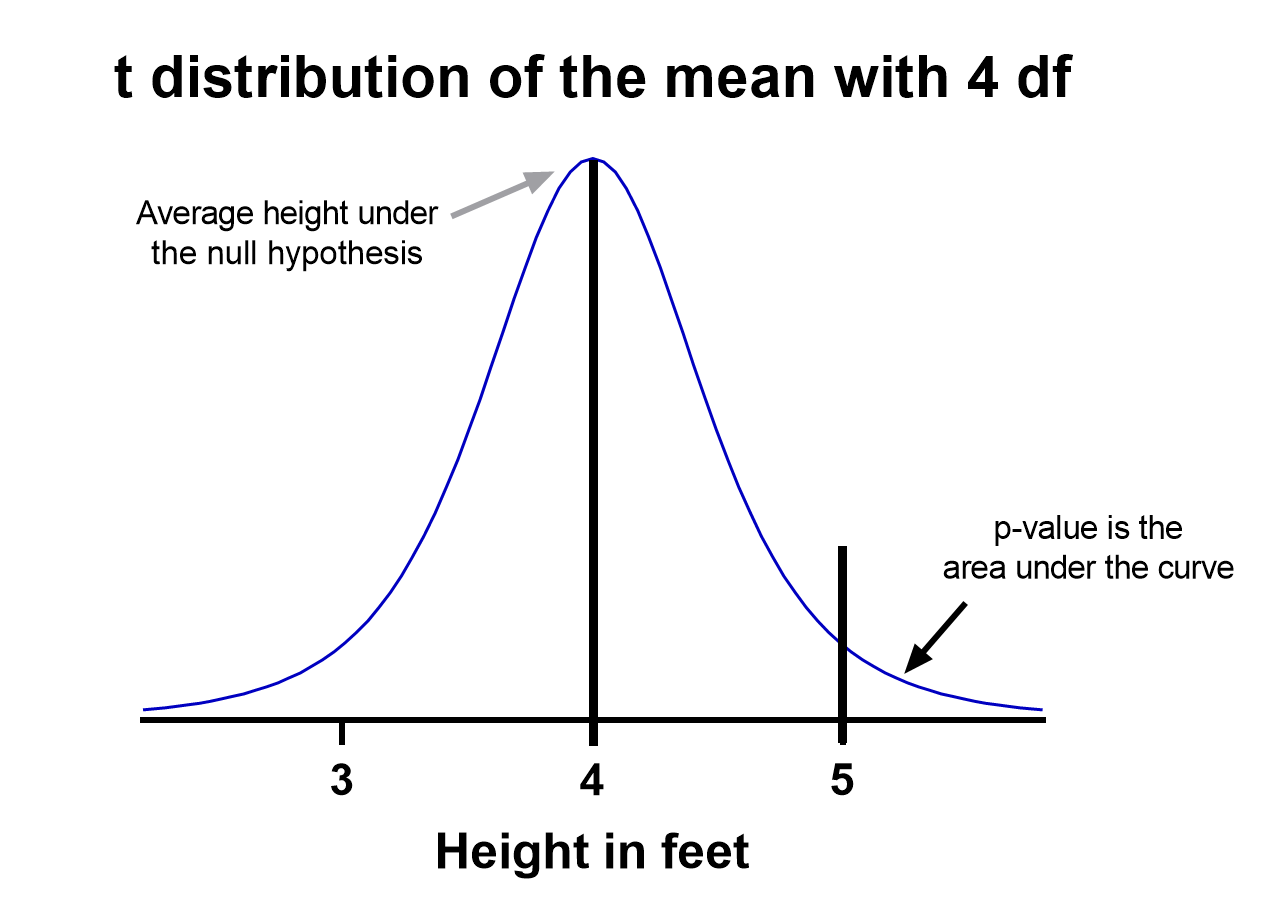
Notice the vertical line at x = 5, which was our sample mean. We (use software to) calculate the area to the right of the vertical line, which gives us the P value (0.09 in this case). Note that because our research question was asking if the average student is greater than four feet, the distribution is centered at four. Since we’re only interested in knowing if the average is greater than four feet, we use a one-tailed test in this case.
Using the standard confidence level of 0.05 with this example, we don’t have evidence that the true average height of sixth graders is taller than 4 feet.
What are the assumptions for t tests?
- One variable of interest : This is not correlation or regression, where you are interested in the relationship between multiple variables. With a t test, you can have different samples, but they are all measuring the same variable (e.g., height).
- Numeric data: You are dealing with a list of measurements that can be averaged. This means you aren’t just counting occurrences in various categories (e.g., eye color or political affiliation).
- Two groups or less: If you have more than two samples of data, a t test is the wrong technique. You most likely need to try ANOVA.
- Random sample : You need a random sample from your statistical “population of interest” in order to draw valid conclusions about the larger population. If your population is so small that you can measure everything, then you have a “census” and don’t need statistics. This is because you don’t need to estimate the truth, since you have measured the truth without variability.
- Normally Distributed : The smaller your sample size, the more important it is that your data come from a normal, Gaussian distribution bell curve. If you have reason to believe that your data are not normally distributed, consider nonparametric t test alternatives . This isn’t necessary for larger samples (usually 25 or 30 unless the data is heavily skewed). The reason is that the Central Limit Theorem applies in this case, which says that even if the distribution of your data is not normal, the distribution of the mean of your data is, so you can use a z-test rather than a t test.
How do I know which t test to use?
There are many types of t tests to choose from, but you don’t necessarily have to understand every detail behind each option.
You just need to be able to answer a few questions, which will lead you to pick the right t test. To that end, we put together this workflow for you to figure out which test is appropriate for your data.
Do you have one or two samples?
Are you comparing the means of two different samples, or comparing the mean from one sample to a fixed value? An example research question is, “Is the average height of my sample of sixth grade students greater than four feet?”
If you only have one sample of data, you can click here to skip to a one-sample t test example, otherwise your next step is to ask:
Are observations in the two samples matched up or related in some way?
This could be as before-and-after measurements of the same exact subjects, or perhaps your study split up “pairs” of subjects (who are technically different but share certain characteristics of interest) into the two samples. The same variable is measured in both cases.
If so, you are looking at some kind of paired samples t test . The linked section will help you dial in exactly which one in that family is best for you, either difference (most common) or ratio.
If you aren’t sure paired is right, ask yourself another question:
Are you comparing different observations in each of the two samples?
If the answer is yes, then you have an unpaired or independent samples t test. The two samples should measure the same variable (e.g., height), but are samples from two distinct groups (e.g., team A and team B).
The goal is to compare the means to see if the groups are significantly different. For example, “Is the average height of team A greater than team B?” Unlike paired, the only relationship between the groups in this case is that we measured the same variable for both. There are two versions of unpaired samples t tests (pooled and unpooled) depending on whether you assume the same variance for each sample.
Have you run the same experiment multiple times on the same subject/observational unit?
If so, then you have a nested t test (unless you have more than two sample groups). This is a trickier concept to understand. One example is if you are measuring how well Fertilizer A works against Fertilizer B. Let’s say you have 12 pots to grow plants in (6 pots for each fertilizer), and you grow 3 plants in each pot.
In this case you have 6 observational units for each fertilizer, with 3 subsamples from each pot. You would want to analyze this with a nested t test . The “nested” factor in this case is the pots. It’s important to note that we aren’t interested in estimating the variability within each pot, we just want to take it into account.
You might be tempted to run an unpaired samples t test here, but that assumes you have 6*3 = 18 replicates for each fertilizer. However, the three replicates within each pot are related, and an unpaired samples t test wouldn’t take that into account.
What if none of these sound like my experiment?
If you’re not seeing your research question above, note that t tests are very basic statistical tools. Many experiments require more sophisticated techniques to evaluate differences. If the variable of interest is a proportion (e.g., 10 of 100 manufactured products were defective), then you’d use z-tests. If you take before and after measurements and have more than one treatment (e.g., control vs a treatment diet), then you need ANOVA.
How do I perform a t test using software?
If you’re wondering how to do a t test, the easiest way is with statistical software such as Prism or an online t test calculator .
If you’re using software, then all you need to know is which t test is appropriate ( use the workflow here ) and understand how to interpret the output. To do that, you’ll also need to:
- Determine whether your test is one or two-tailed
- Choose the level of significance
Is my test one or two-tailed?
Whether or not you have a one- or two-tailed test depends on your research hypothesis. Choosing the appropriately tailed test is very important and requires integrity from the researcher. This is because you have more “power” with one-tailed tests, meaning that you can detect a statistically significant difference more easily. Unless you have written out your research hypothesis as one directional before you run your experiment, you should use a two-tailed test.
Two-tailed tests
Two-tailed tests are the most common, and they are applicable when your research question is simply asking, “is there a difference?”
One-tailed tests
Contrast that with one-tailed tests, where the research questions are directional, meaning that either the question is, “is it greater than ” or the question is, “is it less than ”. These tests can only detect a difference in one direction.
Choosing the level of significance
All t tests estimate whether a mean of a population is different than some other value, and with all estimates come some variability, or what statisticians call “error.” Before analyzing your data, you want to choose a level of significance, usually denoted by the Greek letter alpha, 𝛼. The scientific standard is setting alpha to be 0.05.
An alpha of 0.05 results in 95% confidence intervals, and determines the cutoff for when P values are considered statistically significant.
One sample t test
If you only have one sample of a list of numbers, you are doing a one-sample t test. All you are interested in doing is comparing the mean from this group with some known value to test if there is evidence, that it is significantly different from that standard. Use our free one-sample t test calculator for this.
A one sample t test example research question is, “Is the average fifth grader taller than four feet?”
It is the simplest version of a t test, and has all sorts of applications within hypothesis testing. Sometimes the “known value” is called the “null value”. While the null value in t tests is often 0, it could be any value. The name comes from being the value which exactly represents the null hypothesis, where no significant difference exists.
Any time you know the exact number you are trying to compare your sample of data against, this could work well. And of course: it can be either one or two-tailed.
One sample t test formula
Statistical software handles this for you, but if you want the details, the formula for a one sample t test is:
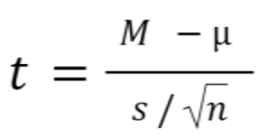
- M: Calculated mean of your sample
- μ: Hypothetical mean you are testing against
- s: The standard deviation of your sample
- n: The number of observations in your sample.
In a one-sample t test, calculating degrees of freedom is simple: one less than the number of objects in your dataset (you’ll see it written as n-1 ).
Example of a one sample t test
For our example within Prism, we have a dataset of 12 values from an experiment labeled “% of control”. Perhaps these are heights of a sample of plants that have been treated with a new fertilizer. A value of 100 represents the industry-standard control height. Likewise, 123 represents a plant with a height 123% that of the control (that is, 23% larger).
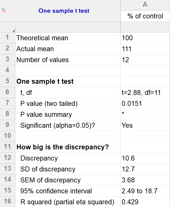
We’ll perform a two-tailed, one-sample t test to see if plants are shorter or taller on average with the fertilizer. We will use a significance threshold of 0.05. Here is the output:
You can see in the output that the actual sample mean was 111. Is that different enough from the industry standard (100) to conclude that there is a statistical difference?
The quick answer is yes, there’s strong evidence that the height of the plants with the fertilizer is greater than the industry standard (p=0.015). The nice thing about using software is that it handles some of the trickier steps for you. In this case, it calculates your test statistic (t=2.88), determines the appropriate degrees of freedom (11), and outputs a P value.
More informative than the P value is the confidence interval of the difference, which is 2.49 to 18.7. The confidence interval tells us that, based on our data, we are confident that the true difference between our sample and the baseline value of 100 is somewhere between 2.49 and 18.7. As long as the difference is statistically significant, the interval will not contain zero.
You can follow these tips for interpreting your own one-sample test.
Graphing a one-sample t test
For some techniques (like regression), graphing the data is a very helpful part of the analysis. For t tests, making a chart of your data is still useful to spot any strange patterns or outliers, but the small sample size means you may already be familiar with any strange things in your data.
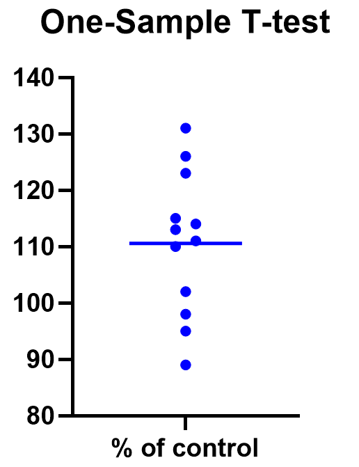
Here we have a simple plot of the data points, perhaps with a mark for the average. We’ve made this as an example, but the truth is that graphing is usually more visually telling for two-sample t tests than for just one sample.
Two sample t tests
There are several kinds of two sample t tests, with the two main categories being paired and unpaired (independent) samples.
Paired samples t test
In a paired samples t test, also called dependent samples t test, there are two samples of data, and each observation in one sample is “paired” with an observation in the second sample. The most common example is when measurements are taken on each subject before and after a treatment. A paired t test example research question is, “Is there a statistical difference between the average red blood cell counts before and after a treatment?”
Having two samples that are closely related simplifies the analysis. Statistical software, such as this paired t test calculator , will simply take a difference between the two values, and then compare that difference to 0.
In some (rare) situations, taking a difference between the pairs violates the assumptions of a t test, because the average difference changes based on the size of the before value (e.g., there’s a larger difference between before and after when there were more to start with). In this case, instead of using a difference test, use a ratio of the before and after values, which is referred to as ratio t tests .
Paired t test formula
The formula for paired samples t test is:
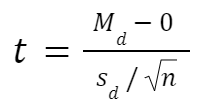
- Md: Mean difference between the samples
- sd: The standard deviation of the differences
- n: The number of differences
Degrees of freedom are the same as before. If you’re studying for an exam, you can remember that the degrees of freedom are still n-1 (not n-2) because we are converting the data into a single column of differences rather than considering the two groups independently.
Also note that the null value here is simply 0. There is no real reason to include “minus 0” in an equation other than to illustrate that we are still doing a hypothesis test. After you take the difference between the two means, you are comparing that difference to 0.
For our example data, we have five test subjects and have taken two measurements from each: before (“control”) and after a treatment (“treated”). If we set alpha = 0.05 and perform a two-tailed test, we observe a statistically significant difference between the treated and control group (p=0.0160, t=4.01, df = 4). We are 95% confident that the true mean difference between the treated and control group is between 0.449 and 2.47.
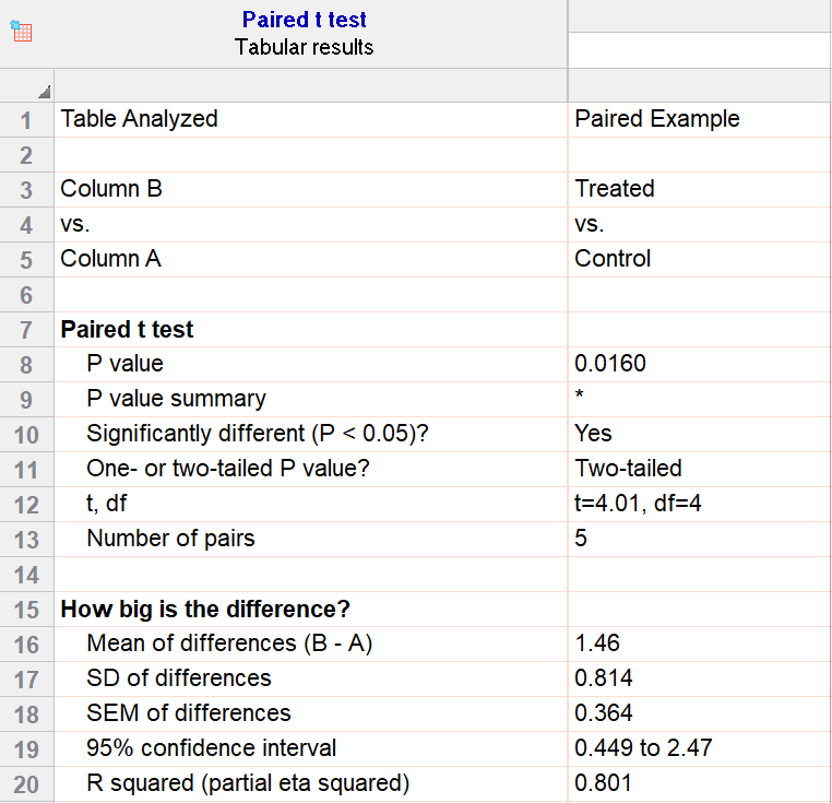
Graphing a paired t test
The significant result of the P value suggests evidence that the treatment had some effect, and we can also look at this graphically. The lines that connect the observations can help us spot a pattern, if it exists. In this case the lines show that all observations increased after treatment. While not all graphics are this straightforward, here it is very consistent with the outcome of the t test.
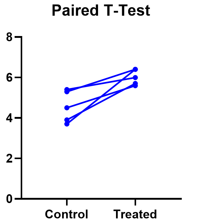
Prism’s estimation plot is even more helpful because it shows both the data (like above) and the confidence interval for the difference between means. You can easily see the evidence of significance since the confidence interval on the right does not contain zero.
Here are some more graphing tips for paired t tests .
Unpaired samples t test
Unpaired samples t test, also called independent samples t test, is appropriate when you have two sample groups that aren’t correlated with one another. A pharma example is testing a treatment group against a control group of different subjects. Compare that with a paired sample, which might be recording the same subjects before and after a treatment.
With unpaired t tests, in addition to choosing your level of significance and a one or two tailed test, you need to determine whether or not to assume that the variances between the groups are the same or not. If you assume equal variances, then you can “pool” the calculation of the standard error between the two samples. Otherwise, the standard choice is Welch’s t test which corrects for unequal variances. This choice affects the calculation of the test statistic and the power of the test, which is the test’s sensitivity to detect statistical significance.
It’s best to choose whether or not you’ll use a pooled or unpooled (Welch’s) standard error before running your experiment, because the standard statistical test is notoriously problematic. See more details about unequal variances here .
As long as you’re using statistical software, such as this two-sample t test calculator , it’s just as easy to calculate a test statistic whether or not you assume that the variances of your two samples are the same. If you’re doing it by hand, however, the calculations get more complicated with unequal variances.
Unpaired (independent) samples t test formula
The general two-sample t test formula is:
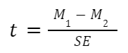
- M1 and M2: Two means you are comparing, one from each dataset
- SE : The combined standard error of the two samples (calculated using pooled or unpooled standard error)
The denominator (standard error) calculation can be complicated, as can the degrees of freedom. If the groups are not balanced (the same number of observations in each), you will need to account for both when determining n for the test as a whole.
As an example for this family, we conduct a paired samples t test assuming equal variances (pooled). Based on our research hypothesis, we’ll conduct a two-tailed test, and use alpha=0.05 for our level of significance. Our samples were unbalanced, with two samples of 6 and 5 observations respectively.
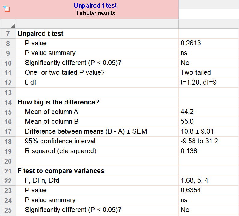
The P value (p=0.261, t = 1.20, df = 9) is higher than our threshold of 0.05. We have not found sufficient evidence to suggest a significant difference. You can see the confidence interval of the difference of the means is -9.58 to 31.2.
Note that the F-test result shows that the variances of the two groups are not significantly different from each other.
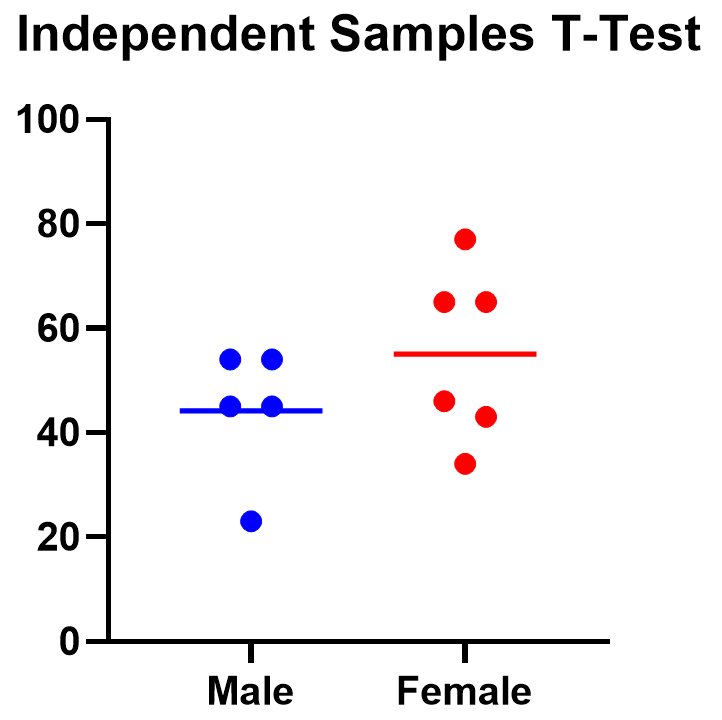
Graphing an unpaired samples t test
For an unpaired samples t test, graphing the data can quickly help you get a handle on the two groups and how similar or different they are. Like the paired example, this helps confirm the evidence (or lack thereof) that is found by doing the t test itself.
Below you can see that the observed mean for females is higher than that for males. But because of the variability in the data, we can’t tell if the means are actually different or if the difference is just by chance.
Nonparametric alternatives for t tests
If your data comes from a normal distribution (or something close enough to a normal distribution), then a t test is valid. If that assumption is violated, you can use nonparametric alternatives.
T tests evaluate whether the mean is different from another value, whereas nonparametric alternatives compare either the median or the rank. Medians are well-known to be much more robust to outliers than the mean.
The downside to nonparametric tests is that they don’t have as much statistical power, meaning a larger difference is required in order to determine that it’s statistically significant.
Wilcoxon signed-rank test
The Wilcoxon signed-rank test is the nonparametric cousin to the one-sample t test. This compares a sample median to a hypothetical median value. It is sometimes erroneously even called the Wilcoxon t test (even though it calculates a “W” statistic).
And if you have two related samples, you should use the Wilcoxon matched pairs test instead. The two versions of Wilcoxon are different, and the matched pairs version is specifically for comparing the median difference for paired samples.
Mann-Whitney and Kolmogorov-Smirnov tests
For unpaired (independent) samples, there are multiple options for nonparametric testing. Mann-Whitney is more popular and compares the mean ranks (the ordering of values from smallest to largest) of the two samples. Mann-Whitney is often misrepresented as a comparison of medians, but that’s not always the case. Kolmogorov-Smirnov tests if the overall distributions differ between the two samples.
More t test FAQs
What is the formula for a t test.
The exact formula depends on which type of t test you are running, although there is a basic structure that all t tests have in common. All t test statistics will have the form:
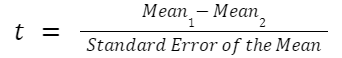
- t : The t test statistic you calculate for your test
- Mean1 and Mean2: Two means you are comparing, at least 1 from your own dataset
- Standard Error of the Mean : The standard error of the mean , also called the standard deviation of the mean, which takes into account the variance and size of your dataset
The exact formula for any t test can be slightly different, particularly the calculation of the standard error. Not only does it matter whether one or two samples are being compared, the relationship between the samples can make a difference too.
What is a t-distribution?
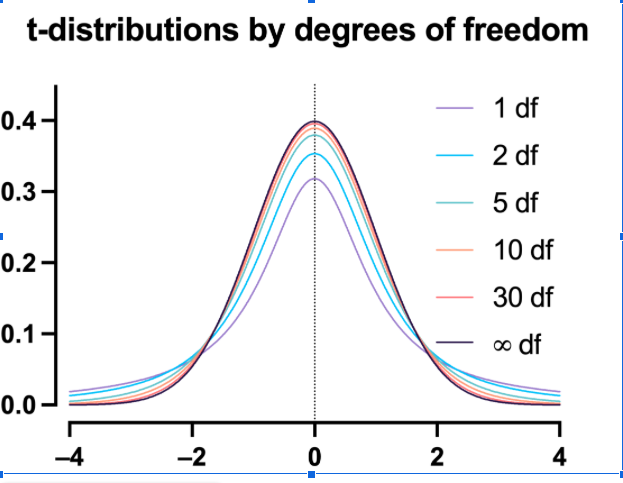
A t-distribution is similar to a normal distribution. It’s a bell-shaped curve, but compared to a normal it has fatter tails, which means that it’s more common to observe extremes. T-distributions are identified by the number of degrees of freedom. The higher the number, the closer the t-distribution gets to a normal distribution. After about 30 degrees of freedom, a t and a standard normal are practically the same.
What are degrees of freedom?
Degrees of freedom are a measure of how large your dataset is. They aren’t exactly the number of observations, because they also take into account the number of parameters (e.g., mean, variance) that you have estimated.
What is the difference between paired vs unpaired t tests?
Both paired and unpaired t tests involve two sample groups of data. With a paired t test, the values in each group are related (usually they are before and after values measured on the same test subject). In contrast, with unpaired t tests, the observed values aren’t related between groups. An unpaired, or independent t test, example is comparing the average height of children at school A vs school B.
When do I use a z-test versus a t test?
Z-tests, which compare data using a normal distribution rather than a t-distribution, are primarily used for two situations. The first is when you’re evaluating proportions (number of failures on an assembly line). The second is when your sample size is large enough (usually around 30) that you can use a normal approximation to evaluate the means.
When should I use ANOVA instead of a t test?
Use ANOVA if you have more than two group means to compare.
What are the differences between t test vs chi square?
Chi square tests are used to evaluate contingency tables , which record a count of the number of subjects that fall into particular categories (e.g., truck, SUV, car). t tests compare the mean(s) of a variable of interest (e.g., height, weight).
What are P values?
P values are the probability that you would get data as or more extreme than the observed data given that the null hypothesis is true. It’s a mouthful, and there are a lot of issues to be aware of with P values.
What are t test critical values?
Critical values are a classical form (they aren’t used directly with modern computing) of determining if a statistical test is significant or not. Historically you could calculate your test statistic from your data, and then use a t-table to look up the cutoff value (critical value) that represented a “significant” result. You would then compare your observed statistic against the critical value.
How do I calculate degrees of freedom for my t test?
In most practical usage, degrees of freedom are the number of observations you have minus the number of parameters you are trying to estimate. The calculation isn’t always straightforward and is approximated for some t tests.
Statistical software calculates degrees of freedom automatically as part of the analysis, so understanding them in more detail isn’t needed beyond assuaging any curiosity.
Perform your own t test
Are you ready to calculate your own t test? Start your 30 day free trial of Prism and get access to:
- A step by step guide on how to perform a t test
- Sample data to save you time
- More tips on how Prism can help your research
With Prism, in a matter of minutes you learn how to go from entering data to performing statistical analyses and generating high-quality graphs.
- History & Society
- Science & Tech
- Biographies
- Animals & Nature
- Geography & Travel
- Arts & Culture
- Games & Quizzes
- On This Day
- One Good Fact
- New Articles
- Lifestyles & Social Issues
- Philosophy & Religion
- Politics, Law & Government
- World History
- Health & Medicine
- Browse Biographies
- Birds, Reptiles & Other Vertebrates
- Bugs, Mollusks & Other Invertebrates
- Environment
- Fossils & Geologic Time
- Entertainment & Pop Culture
- Sports & Recreation
- Visual Arts
- Demystified
- Image Galleries
- Infographics
- Top Questions
- Britannica Kids
- Saving Earth
- Space Next 50
- Student Center
- Where was science invented?
- When did science begin?

Student’s t-test
Our editors will review what you’ve submitted and determine whether to revise the article.
- National Center for Biotechnology Information - PubMed Central - Application of Student's t-test, Analysis of Variance, and Covariance
- BCcampus Publishing - The t-Test
- University of Missouri System - Introduction to t Tests
- University of California - Department of Statistics - t-Tests
- Rice University - Foundations of Linguistics - 'Student's' t Test (For Independent Samples)
- Statistics LibreTexts - The Independent Samples t-test (Student Test)
Student’s t-test , in statistics , a method of testing hypotheses about the mean of a small sample drawn from a normally distributed population when the population standard deviation is unknown.
In 1908 William Sealy Gosset, an Englishman publishing under the pseudonym Student, developed the t -test and t distribution. (Gosset worked at the Guinness brewery in Dublin and found that existing statistical techniques using large samples were not useful for the small sample sizes that he encountered in his work.) The t distribution is a family of curves in which the number of degrees of freedom (the number of independent observations in the sample minus one) specifies a particular curve. As the sample size (and thus the degrees of freedom) increases, the t distribution approaches the bell shape of the standard normal distribution . In practice, for tests involving the mean of a sample of size greater than 30, the normal distribution is usually applied.
It is usual first to formulate a null hypothesis , which states that there is no effective difference between the observed sample mean and the hypothesized or stated population mean—i.e., that any measured difference is due only to chance . In an agricultural study, for example, the null hypothesis could be that an application of fertilizer has had no effect on crop yield, and an experiment would be performed to test whether it has increased the harvest. In general, a t -test may be either two-sided (also termed two-tailed), stating simply that the means are not equivalent, or one-sided, specifying whether the observed mean is larger or smaller than the hypothesized mean. The test statistic t is then calculated. If the observed t -statistic is more extreme than the critical value determined by the appropriate reference distribution, the null hypothesis is rejected. The appropriate reference distribution for the t -statistic is the t distribution. The critical value depends on the significance level of the test (the probability of erroneously rejecting the null hypothesis).

A second application of the t distribution tests the hypothesis that two independent random samples have the same mean. The t distribution can also be used to construct confidence intervals for the true mean of a population (the first application) or for the difference between two sample means (the second application). See also interval estimation .

- Get new issue alerts Get alerts
- Submit a Manuscript
Secondary Logo
Journal logo.
Colleague's E-mail is Invalid
Your message has been successfully sent to your colleague.
Save my selection
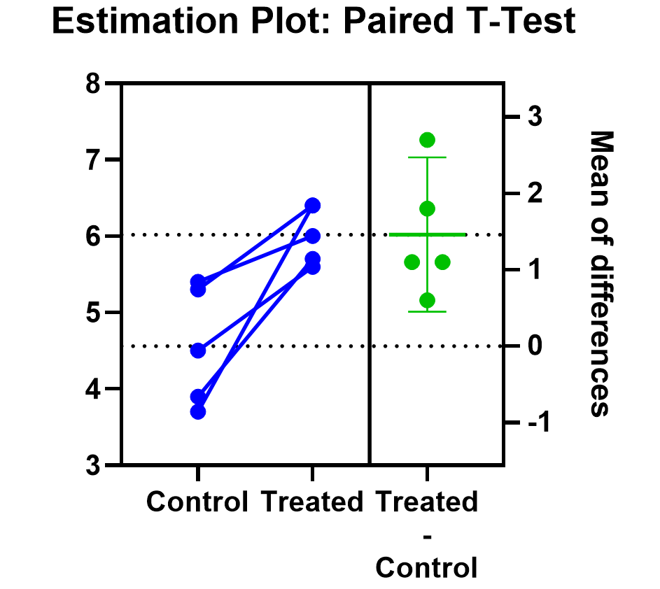
Commonly Used t -tests in Medical Research
Pandey, R. M.
Department of Biostatistics, All India Institute of Medical Sciences, New Delhi, India
Address for correspondence: Dr. R.M. Pandey, Department of Biostatistics, All India Institute of Medical Sciences, New Delhi, India. E-mail: [email protected]
This is an open access journal, and articles are distributed under the terms of the Creative Commons Attribution-NonCommercial-ShareAlike 4.0 License, which allows others to remix, tweak, and build upon the work non-commercially, as long as appropriate credit is given and the new creations are licensed under the identical terms.
Student's t -test is a method of testing hypotheses about the mean of a small sample drawn from a normally distributed population when the population standard deviation is unknown. In 1908 William Sealy Gosset, an Englishman publishing under the pseudonym Student, developed the t -test. This article discusses the types of T test and shows a simple way of doing a T test.
INTRODUCTION
To draw some conclusion about a population parameter (true result of any phenomena in the population) using the information contained in a sample, two approaches of statistical inference are used, that is, confidence interval (range of results likely to be obtained, usually, 95% of the times) and hypothesis testing, to find how often the observed finding could be due to chance alone, reported by P value which is the probability of obtaining the result as extreme as observed under null hypothesis. Statistical tests used for hypothesis testing are broadly classified into two groups, that is, parametric tests and nonparametric tests. In parametric tests, some assumption is made about the distribution of population from which the sample is drawn. In all parametric tests, the distribution of quantitative variable in the population is assumed to be normally distributed. As one does not have access to the population values to say normal or nonnormal, assumption of normality is made based on the sample values. Nonparametric statistical methods are also known as distribution-free methods or methods based on ranks where no assumptions are made about the distribution of variable in the population.
The family of t -tests falls in the category of parametric statistical tests where the mean value(s) is (are) compared against a hypothesized value. In hypothesis testing of any statistic (summary), for example, mean or proportion, the hypothesized value of the statistic is specified while the population variance is not specified, in such a situation, available information is only about variability in the sample. Therefore, to compute the standard error (measure of variability of the statistic of interest which is always in the denominator of the test statistic), it is considered reasonable to use sample standard deviation. William Sealy Gosset, a chemist working for a brewery in Dublin Ireland introduced the t -statistic. As per the company policy, chemists were not allowed to publish their findings, so Gosset published his mathematical work under the pseudonym “Student,” his pen name. The Student's t -test was published in the journal Biometrika in 1908.[ 1 , 2 ]
In medical research, various t -tests and Chi-square tests are the two types of statistical tests most commonly used. In any statistical hypothesis testing situation, if the test statistic follows a Student's t -test distribution under null hypothesis, it is a t -test. Most frequently used t -tests are: For comparison of mean in single sample; two samples related; two samples unrelated tests; and testing of correlation coefficient and regression coefficient against a hypothesized value which is usually zero. In one-sample location test, it is tested whether or not the mean of the population has a value as specified in a null hypothesis; in two independent sample location test, equality of means of two populations is tested; to compare the mean delta (difference between two related samples) against hypothesized value of zero in a null hypothesis, also known as paired t -test or repeated-measures t -test; and, to test whether or not the slope of a regression line differs significantly from zero. For a binary variable (such as cure, relapse, hypertension, diabetes, etc.,) which is either yes or no for a subject, if we take 1 for yes and 0 for no and consider this as a score attached to each study subject then the sample proportion (p) and the sample mean would be the same. Therefore, the approach of t -test for mean can be used for proportion as well.
The focus here is on describing a situation where a particular t -test would be used. This would be divided into t -tests used for testing: (a) Mean/proportion in one sample, (b) mean/proportion in two unrelated samples, (c) mean/proportion in two related samples, (d) correlation coefficient, and (e) regression coefficient. The process of hypothesis testing is same for any statistical test: Formulation of null and alternate hypothesis; identification and computation of test statistics based on sample values; deciding of alpha level, one-tailed or two-tailed test; rejection or acceptance of null hypothesis by comparing the computed test statistic with the theoretical value of “ t ” from the t -distribution table corresponding to given degrees of freedom. In hypothesis testing, P value is reported as P < 0.05. However, in significance testing, the exact P value is reported so that the reader is in a better position to judge the level of statistical significance.
- t -test for one sample: For example, in a random sample of 30 hypertensive males, the observed mean body mass index (BMI) is 27.0 kg/m 2 and the standard deviation is 4.0. Also, suppose it is known that the mean BMI in nonhypertensive males is 25 kg/m 2 . If the question is to know whether or not these 30 observations could have come from a population with a mean of 25 kg/m 2 . To determine this, one sample t -test is used with the null hypothesis H0: Mean = 25, against alternate hypothesis of H1: Mean ≠ 25. Since the standard deviation of the hypothesized population is not known, therefore, t -test would be appropriate; otherwise, Z -test would have been used
- t -test for two related samples: Two samples can be regarded as related in a pre- and post-design (self-pairing) or in two groups where the subjects have been matched on a third factor a known confounder (artificial pairing). In a pre- and post–design, each subject is used as his or her own control. For example, an investigator wants to assess effect of an intervention in reducing systolic blood pressure (SBP) in a pre- and post-design. Here, for each patient, there would be two observations of SBP, that is, before and after. Here instead of individual observations, difference between pairs of observations would be of interest and the problem reduces to one-sample situation where the null hypothesis would be to test the mean difference in SBP equal to zero against the alternate hypothesis of mean SBP being not equal to zero. The underlying assumption for using paired t -test is that under the null hypothesis the population of difference in normally distributed and this can be judged using the sample values. Using the mean difference and the standard error of the mean difference, 95% confidence interval can be computed. The other situation of the two sample being related is the two group matched design. For example, in a case–control study to assess association between smoking and hypertension, both hypertensive and nonhypertensive are matched on some third factor, say obesity, in a pair-wise manner. Same approach of paired analysis would be used. In this situation, cases and controls are different subjects. However, they are related by the factor
- t -test for two independent samples: To test the null hypothesis that the means of two populations are equal; Student's t -test is used provided the variances of the two populations are equal and the two samples are assumed to be random sample. When this assumption of equality of variance is not fulfilled, the form of the test used is a modified t -test. These tests are also known as two-sample independent t -tests with equal variance or unequal variance, respectively. The only difference in the two statistical tests lies in the denominator, that is, in determining the pooled variance. Prior to choosing t -test for equal or unequal variance, very often a test of variance is carried out to compare the two variances. It is recommended that this should be avoided.[ 3 ] Using a modified t -test even in a situation when the variances are equal, has high power, therefore, to compare the means in the two unrelated groups, using a modified t -test is sufficient.[ 4 ] When there are more than two groups, use of multiple t -test (for each pair of groups) is incorrect because it may give false-positive result, hence, in such situations, one-way analysis of variance (ANOVA), followed by correction in P value for multiple comparisons ( post-hoc ANOVA), if required, is used to test the equality of more than two means as the null hypothesis, ensuring that the total P value of all the pair-wise does not exceed 0.05
- t -test for correlation coefficient: To quantify the strength of relationship between two quantitative variables, correlation coefficient is used. When both the variables follow normal distribution, Pearson's correlation coefficient is computed; and when one or both of the variables are nonnormal or ordinal, Spearman's rank correlation coefficient (based on ranks) are used. For both these measures, in the case of no linear correlation, null value is zero and under null hypothesis, the test statistic follows t -distribution and therefore, t -test is used to find out whether or not the Pearson's/Spearman's rank correlation coefficient is significantly different from zero
- Regression coefficient: Regression methods are used to model a relationship between a factor and its potential predictors. Type of regression method to be used depends on the type of dependent/outcome/effect variable. Three most commonly used regression methods are multiple linear regression, multiple logistic regression, and Cox regression. The form of the dependent variable in these three methods is quantitative, categorical, and time to an event, respectively. A multiple linear regression would be of the form Y = a + b1×1 + b2×2 +…, where Y is the outcome and X's are the potential covariates. In logistic and Cox regression, the equation is nonlinear and using transformation the equation is converted into linear equation because it is easy to obtain unknowns in the linear equation using sample observations. The computed values of a and b vary from sample to sample. Therefore, to test the null hypothesis that there is no relationship between X and Y, t -test, which is the coefficient divided by its standard error, is used to determine the P value. This is also commonly referred to as Wald t -test and using the numerator and denominator of the Wald t -statistic, 95% confidence interval is computed as coefficient ± 1.96 (standard error of the coefficient).
The above is an illustration of the most common situations where t -test is used. With availability of software, computation is not the issue anymore. Any software where basic statistical methods are provided will have these tests. All one needs to do is to identify the t -test to be used in a given situation, arrange the data in the manner required by the particular software, and use mouse to perform the test and report the following: Number of observations, summary statistic, P value, and the 95% confidence interval of summary statistic of interest.
USING AN ONLINE CALCULATOR TO COMPUTE T -STATISTICS
In addition to the statistical software, you can also use online calculators for calculating the t -statistics, P values, 95% confidence interval, etc., Various online calculators are available over the World Wide Web. However, for explaining how to use these calculators, a brief description is given below. A link to one of the online calculator available over the internet is http://www.graphpad.com/quickcalcs/ .
- Step 1: The first screen that will appear by typing this URL in address bar will be somewhat as shown in Figure 1 .
- Step 2: Check on the continuous data option as shown in Figure 1 and press continue
- Step 3: On pressing the continue tab, you will be guided to another screen as shown in Figure 2 .
- Step 4: For calculating the one-sample t -statistic, click on the one-sample t -test. Compare observed and expected means option as shown in Figure 2 and press continue. For comparing the two means as usually done in the paired t -test for related samples and two-sample independent t -test, click on the t -test to compare two means option.
- Step 5: After pressing the continue tab, you will be guided to another screen as shown in Figure 3 . Choose the data entry format, like for the BMI and hypertensive males' example given for the one-sample t -test, we have n, mean, and standard deviation of the sample that has to be compared with the hypothetical mean value of 25 kg/m 2 . Enter the values in the calculator and set the hypothetical value to 25 and then press the calculate now tab. Refer to [ Figure 3 ] for details
- Step 6: On pressing the calculate now tab, you will be guided to next screen as shown in Figure 4 , which will give you the results of your one-sample t -test. It can be seen from the results given in Figure 4 that the P value for our one-sample t -test is 0.0104. 95% confidence interval is 0.51–3.49 and one-sample t -statistics is 2.7386.

Similarly online t -test calculators can be used to calculate the paired t -test ( t -test for two related samples) and t -test for two independent samples. You just need to look that in what format you are having the data and a basic knowledge of in which condition which test has to be applied and what is the correct form for entering the data in the calculator.
Financial support and sponsorship
Conflicts of interest.
There are no conflicts of interest.
- Cited Here |
Student's T test; method; William Gosset
- + Favorites
- View in Gallery
Readers Of this Article Also Read
Types of variables in medical research, the story of heart transplantation: from cape town to cape comorin, the odds ratio: principles and applications, how to use medical search engines, tools for placing research in context.
JMP | Statistical Discovery.™ From SAS.
Statistics Knowledge Portal
A free online introduction to statistics
What is a t- test?
A t -test (also known as Student's t -test) is a tool for evaluating the means of one or two populations using hypothesis testing. A t-test may be used to evaluate whether a single group differs from a known value (a one-sample t-test), whether two groups differ from each other (an independent two-sample t-test), or whether there is a significant difference in paired measurements (a paired, or dependent samples t-test).
How are t -tests used?
First, you define the hypothesis you are going to test and specify an acceptable risk of drawing a faulty conclusion. For example, when comparing two populations, you might hypothesize that their means are the same, and you decide on an acceptable probability of concluding that a difference exists when that is not true. Next, you calculate a test statistic from your data and compare it to a theoretical value from a t- distribution. Depending on the outcome, you either reject or fail to reject your null hypothesis.
What if I have more than two groups?
You cannot use a t -test. Use a multiple comparison method. Examples are analysis of variance ( ANOVA ) , Tukey-Kramer pairwise comparison, Dunnett's comparison to a control, and analysis of means (ANOM).
t -Test assumptions
While t -tests are relatively robust to deviations from assumptions, t -tests do assume that:
- The data are continuous.
- The sample data have been randomly sampled from a population.
- There is homogeneity of variance (i.e., the variability of the data in each group is similar).
- The distribution is approximately normal.
For two-sample t -tests, we must have independent samples. If the samples are not independent, then a paired t -test may be appropriate.
Types of t -tests
There are three t -tests to compare means: a one-sample t -test, a two-sample t -test and a paired t -test. The table below summarizes the characteristics of each and provides guidance on how to choose the correct test. Visit the individual pages for each type of t -test for examples along with details on assumptions and calculations.
| test | test | test | |
|---|---|---|---|
| Synonyms | Student’s -test | -test test -test -test -test | test -test |
| Number of variables | One | Two | Two |
| Type of variable | |||
| Purpose of test | Decide if the population mean is equal to a specific value or not | Decide if the population means for two different groups are equal or not | Decide if the difference between paired measurements for a population is zero or not |
| Example: test if... | Mean heart rate of a group of people is equal to 65 or not | Mean heart rates for two groups of people are the same or not | Mean difference in heart rate for a group of people before and after exercise is zero or not |
| Estimate of population mean | Sample average | Sample average for each group | Sample average of the differences in paired measurements |
| Population standard deviation | Unknown, use sample standard deviation | Unknown, use sample standard deviations for each group | Unknown, use sample standard deviation of differences in paired measurements |
| Degrees of freedom | Number of observations in sample minus 1, or: n–1 | Sum of observations in each sample minus 2, or: n + n – 2 | Number of paired observations in sample minus 1, or: n–1 |
The table above shows only the t -tests for population means. Another common t -test is for correlation coefficients . You use this t -test to decide if the correlation coefficient is significantly different from zero.
One-tailed vs. two-tailed tests
When you define the hypothesis, you also define whether you have a one-tailed or a two-tailed test. You should make this decision before collecting your data or doing any calculations. You make this decision for all three of the t -tests for means.
To explain, let’s use the one-sample t -test. Suppose we have a random sample of protein bars, and the label for the bars advertises 20 grams of protein per bar. The null hypothesis is that the unknown population mean is 20. Suppose we simply want to know if the data shows we have a different population mean. In this situation, our hypotheses are:
$ \mathrm H_o: \mu = 20 $
$ \mathrm H_a: \mu \neq 20 $
Here, we have a two-tailed test. We will use the data to see if the sample average differs sufficiently from 20 – either higher or lower – to conclude that the unknown population mean is different from 20.
Suppose instead that we want to know whether the advertising on the label is correct. Does the data support the idea that the unknown population mean is at least 20? Or not? In this situation, our hypotheses are:
$ \mathrm H_o: \mu >= 20 $
$ \mathrm H_a: \mu < 20 $
Here, we have a one-tailed test. We will use the data to see if the sample average is sufficiently less than 20 to reject the hypothesis that the unknown population mean is 20 or higher.
See the "tails for hypotheses tests" section on the t -distribution page for images that illustrate the concepts for one-tailed and two-tailed tests.
How to perform a t -test
For all of the t -tests involving means, you perform the same steps in analysis:
- Define your null ($ \mathrm H_o $) and alternative ($ \mathrm H_a $) hypotheses before collecting your data.
- Decide on the alpha value (or α value). This involves determining the risk you are willing to take of drawing the wrong conclusion. For example, suppose you set α=0.05 when comparing two independent groups. Here, you have decided on a 5% risk of concluding the unknown population means are different when they are not.
- Check the data for errors.
- Check the assumptions for the test.
- Perform the test and draw your conclusion. All t -tests for means involve calculating a test statistic. You compare the test statistic to a theoretical value from the t- distribution . The theoretical value involves both the α value and the degrees of freedom for your data. For more detail, visit the pages for one-sample t -test , two-sample t -test and paired t -test .

An official website of the United States government
The .gov means it’s official. Federal government websites often end in .gov or .mil. Before sharing sensitive information, make sure you’re on a federal government site.
The site is secure. The https:// ensures that you are connecting to the official website and that any information you provide is encrypted and transmitted securely.
- Publications
- Account settings
Preview improvements coming to the PMC website in October 2024. Learn More or Try it out now .
- Advanced Search
- Journal List
- Korean J Anesthesiol
- v.68(6); 2015 Dec
T test as a parametric statistic
Tae kyun kim.
Department of Anesthesia and Pain Medicine, Pusan National University School of Medicine, Busan, Korea.
In statistic tests, the probability distribution of the statistics is important. When samples are drawn from population N (µ, σ 2 ) with a sample size of n, the distribution of the sample mean X ̄ should be a normal distribution N (µ, σ 2 / n ). Under the null hypothesis µ = µ 0 , the distribution of statistics z = X ¯ - µ 0 σ / n should be standardized as a normal distribution. When the variance of the population is not known, replacement with the sample variance s 2 is possible. In this case, the statistics X ¯ - µ 0 s / n follows a t distribution ( n-1 degrees of freedom). An independent-group t test can be carried out for a comparison of means between two independent groups, with a paired t test for paired data. As the t test is a parametric test, samples should meet certain preconditions, such as normality, equal variances and independence.
Introduction
A t test is a type of statistical test that is used to compare the means of two groups. It is one of the most widely used statistical hypothesis tests in pain studies [ 1 ]. There are two types of statistical inference: parametric and nonparametric methods. Parametric methods refer to a statistical technique in which one defines the probability distribution of probability variables and makes inferences about the parameters of the distribution. In cases in which the probability distribution cannot be defined, nonparametric methods are employed. T tests are a type of parametric method; they can be used when the samples satisfy the conditions of normality, equal variance, and independence.
T tests can be divided into two types. There is the independent t test, which can be used when the two groups under comparison are independent of each other, and the paired t test, which can be used when the two groups under comparison are dependent on each other. T tests are usually used in cases where the experimental subjects are divided into two independent groups, with one group treated with A and the other group treated with B. Researchers can acquire two types of results for each group (i.e., prior to treatment and after the treatment): preA and postA, and preB and postB. An independent t test can be used for an intergroup comparison of postA and postB or for an intergroup comparison of changes in preA to postA (postA-preA) and changes in preB to postB (postB-preB) ( Table 1 ).
| Treatment A | Treatment B | |||||||
|---|---|---|---|---|---|---|---|---|
| ID | preA | postA | ΔA | ID | preB | postB | ΔB | |
| 1 | 63 | 77 | 14 | 11 | 81 | 101 | 20 | |
| 2 | 69 | 88 | 19 | 12 | 87 | 103 | 16 | |
| 3 | 76 | 90 | 14 | 13 | 77 | 107 | 30 | |
| 4 | 78 | 95 | 17 | 14 | 80 | 114 | 34 | |
| 5 | 80 | 96 | 16 | 15 | 76 | 116 | 40 | |
| 6 | 89 | 96 | 7 | 16 | 86 | 116 | 30 | |
| 7 | 90 | 102 | 12 | 17 | 98 | 116 | 18 | |
| 8 | 92 | 104 | 12 | 18 | 87 | 120 | 33 | |
| 9 | 103 | 110 | 7 | 19 | 105 | 120 | 15 | |
| 10 | 112 | 115 | 3 | 20 | 69 | 127 | 58 | |
ID: individual identification, preA, preB: before the treatment A or B, postA, postB: after the treatment A or B, ΔA, ΔB: difference between before and after the treatment A or B.
On the other hand, paired t tests are used in different experimental environments. For example, the experimental subjects are not divided into two groups, and all of them are treated initially with A. The amount of change (postA-preA) is then measured for all subjects. After all of the effects of A disappear, the subjects are treated with B, and the amount of change (postB-preB) is measured for all of the subjects. A paired t test is used in such crossover test designs to compare the amount of change of A to that of B for the same subjects ( Table 2 ).
| Treatment A | Treatment B | |||||||
|---|---|---|---|---|---|---|---|---|
| ID | preA | postA | ΔA | ID | preB | postB | ΔB | |
| 1 | 63 | 77 | 14 | 1 | 73 | 103 | 30 | |
| 2 | 69 | 88 | 19 | 2 | 74 | 104 | 30 | |
| 3 | 76 | 90 | 14 | 3 | 76 | 107 | 31 | |
| 4 | 78 | 95 | 17 | 4 | 84 | 108 | 24 | |
| 5 | 80 | 96 | 16 | wash out | 5 | 84 | 110 | 26 |
| 6 | 89 | 96 | 7 | 6 | 86 | 110 | 24 | |
| 7 | 90 | 102 | 12 | 7 | 92 | 113 | 21 | |
| 8 | 92 | 104 | 12 | 8 | 95 | 114 | 19 | |
| 9 | 103 | 110 | 7 | 9 | 103 | 118 | 15 | |
| 10 | 112 | 115 | 3 | 10 | 115 | 120 | 5 | |
Statistic and Probability
Statistics is basically about probabilities. A statistical conclusion of a large or small difference between two groups is not based on an absolute standard but is rather an evaluation of the probability of an event. For example, a clinical test is performed to determine whether or not a patient has a certain disease. If the test results are either higher or lower than the standard, clinicians will determine that the patient has the disease despite the fact that the patient may or may not actually have the disease. This conclusion is based on the statistical concept which holds that it is more statistically valid to conclude that the patient has the disease than to declare that the patient is a rare case among people without the disease because such test results are statistically rare in normal people.
The test results and the probability distribution of the results must be known in order for the results to be determined as statistically rare. The criteria for clinical indicators have been established based on data collected from an entire population or at least from a large number of people. Here, we examine a case in which a clinical indicator exhibits a normal distribution with a mean of µ and a variance of σ 2 . If a patient's test result is χ, is this statistically rare against the criteria (e.g., 5 or 1%)? Probability is represented as the surface area in a probability distribution, and the z score that represents either 5 or 1%, near the margins of the distribution, becomes the reference value. The test result χ can be determined to be statistically rare compared to the reference probability if it lies in a more marginal area than the z score, that is, if the value of χ is located in the marginal ends of the distribution ( Fig. 1 ).

This is done to compare one individual's clinical indicator value. This however raises the question of how we would compare the mean of a sample group (consisting of more than one individual) against the population mean. Again, it is meaningless to compare each individual separately; we must compare the means of the two groups. Thus, do we make a statistical inference using only the distribution of the clinical indicators of the entire population and the mean of the sample? No. In order to infer a statistical possibility, we must know the indicator of interest and its probability distribution. In other words, we must know the mean of the sample and the distribution of the mean. We can then determine how far the sample mean varies from the population mean by knowing the sampling distribution of the means.
Sampling Distribution (Sample Mean Distribution)
The sample mean we can get from a study is one of means of all possible samples which could be drawn from a population. This sample mean from a study was already acquired from a real experiment, however, how could we know the distribution of the means of all possible samples including studied sample? Do we need to experiment it over and over again? The simulation in which samples are drawn repeatedly from a population is shown in Fig. 2 . If samples are drawn with sample size n from population of normal distribution (µ, σ 2 ), the sampling distribution shows normal distribution with mean of µ and variance of σ 2 / n . The number of samples affects the shape of the sampling distribution. That is, the shape of the distribution curve becomes a narrower bell curve with a smaller variance as the number of samples increases, because the variance of sampling distribution is σ 2 / n . The formation of a sampling distribution is well explained in Lee et al. [ 2 ] in a form of a figure.

T Distribution
Now that the sampling distribution of the means is known, we can locate the position of the mean of a specific sample against the distribution data. However, one problem remains. As we noted earlier, the sampling distribution exhibits a normal distribution with a variance of σ 2 / n , but in reality we do not know σ 2 , the variance of the population. Therefore, we use the sample variance instead of the population variance to determine the sampling distribution of the mean. The sample variance is defined as follows:
In such cases in which the sample variance is used, the sampling distribution follows a t distribution that depends on the 0degree of freedom of each sample rather than a normal distribution ( Fig. 3 ).

Independent T test
A t test is also known as Student's t test. It is a statistical analysis technique that was developed by William Sealy Gosset in 1908 as a means to control the quality of dark beers. A t test used to test whether there is a difference between two independent sample means is not different from a t test used when there is only one sample (as mentioned earlier). However, if there is no difference in the two sample means, the difference will be close to zero. Therefore, in such cases, an additional statistical test should be performed to verify whether the difference could be said to be equal to zero.
Let's extract two independent samples from a population that displays a normal distribution and compute the difference between the means of the two samples. The difference between the sample means will not always be zero, even if the samples are extracted from the same population, because the sampling process is randomized, which results in a sample with a variety of combinations of subjects. We extracted two samples with a size of 6 from a population N (150, 5 2 ) and found the difference in the means. If this process is repeated 1,000 times, the sampling distribution exhibits the shape illustrated in Fig. 4 . When the distribution is displayed in terms of a histogram and a density line, it is almost identical to the theoretical sampling distribution: N(0, 2 × 5 2 /6) ( Fig. 4 ).

However, it is difficult to define the distribution of the difference in the two sample means because the variance of the population is unknown. If we use the variance of the sample instead, the distribution of the difference of the samples means would follow a t distribution. It should be noted, however, that the two samples display a normal distribution and have an equal variance because they were independently extracted from an identical population that has a normal distribution.
Under the assumption that the two samples display a normal distribution and have an equal variance, the t statistic is as follows:
population mean difference (µ 1 - µ 2 ) was assumed to be 0; thus:
The population variance was unknown and so a pooled variance of the two samples was used:
However, if the population variance is not equal, the t statistic of the t test would be
and the degree of freedom is calculated based on the Welch Satterthwaite equation.
It is apparent that if n 1 and n 2 are sufficiently large, the t statistic resembles a normal distribution ( Fig. 3 ).
A statistical test is performed to verify the position of the difference in the sample means in the sampling distribution of the mean ( Fig. 4 ). It is statistically very rare for the difference in two sample means to lie on the margins of the distribution. Therefore, if the difference does lie on the margins, it is statistically significant to conclude that the samples were extracted from two different populations, even if they were actually extracted from the same population.
Paired T test
Paired t tests are can be categorized as a type of t test for a single sample because they test the difference between two paired results. If there is no difference between the two treatments, the difference in the results would be close to zero; hence, the difference in the sample means used for a paired t test would be 0.
Let's go back to the sampling distribution that was used in the independent t test discussed earlier. The variance of the difference between two independent sample means was represented as the sum of each variance. If the samples were not independent, the variance of the difference of two variables A and B, Var (A-B), can be shown as follows,
where σ 1 2 is the variance of variable A, σ 2 2 is the variance of variable B, and ρ is the correlation coefficient for the two variables. In an independent t test, the correlation coefficient is 0 because the two groups are independent. Thus, it is logical to show the variance of the difference between the two variables simply as the sum of the two variances. However, for paired variables, the correlation coefficient may not equal 0. Thus, the t statistic for two dependent samples must be different, meaning the following t statistic,
must be changed. First, the number of samples are paired; thus, n 1 = n 2 = n , and their variance can be represented as s 1 2 + s 2 2 - 2ρ s 1 s 2 considering the correlation coefficient. Therefore, the t statistic for a paired t test is as follows:
In this equation, the t statistic is increased if the correlation coefficient is greater than 0 because the denominator becomes smaller, which increases the statistical power of the paired t test compared to that of an independent t test. On the other hand, if the correlation coefficient is less than 0, the statistical power is decreased and becomes lower than that of an independent t test. It is important to note that if one misunderstands this characteristic and uses an independent t test when the correlation coefficient is less than 0, the generated results would be incorrect, as the process ignores the paired experimental design.
Assumptions
As previously explained, if samples are extracted from a population that displays a normal distribution but the population variance is unknown, we can use the sample variance to examine the sampling distribution of the mean, which will resemble a t distribution. Therefore, in order to reach a statistical conclusion about a sample mean with a t distribution, certain conditions must be satisfied: the two samples for comparison must be independently sampled from the same population, satisfying the conditions of normality, equal variance, and independence.
Shapiro's test or the Kolmogorov-Smirnov test can be performed to verify the assumption of normality. If the condition of normality is not met, the Wilcoxon rank sum test (Mann-Whitney U test) is used for independent samples, and the Wilcoxon sign rank test is used for paired samples for an additional nonparametric test.
The condition of equal variance is verified using Levene's test or Bartlett's test. If the condition of equal variance is not met, nonparametric test can be performed or the following statistic which follows a t distribution can is used.
However, this statistics has different degree of freedom which was calculated by the Welch-Satterthwaite [ 3 , 4 ] equation.
Owing to user-friendly statistics software programs, the rich pool of statistics information on the Internet, and expert advice from statistics professionals at every hospital, using and processing statistics data is no longer an intractable task. However, it remains the researchers' responsibility to design experiments to fulfill all of the conditions of their statistic methods of choice and to ensure that their statistical assumptions are appropriate. In particular, parametric statistical methods confer reasonable statistical conclusions only when the statistical assumptions are fully met. Some researchers often regard these statistical assumptions inconvenient and neglect them. Even some statisticians argue on the basic assumptions, based on the central limit theory, that sampling distributions display a normal distribution regardless of the fact that the population distribution may or may not follow a normal distribution, and that t tests have sufficient statistical power even if they do not satisfy the condition of normality [ 5 ]. Moreover, they contend that the condition of equal variance is not so strict because even if there is a ninefold difference in the variance, the α level merely changes from 0.5 to 0.6 [ 6 ]. However, the arguments regarding the conditions of normality and the limit to which the condition of equal variance may be violated are still bones of contention. Therefore, researchers who unquestioningly accept these arguments and neglect the basic assumptions of a t test when submitting papers will face critical comments from editors. Moreover, it will be difficult to persuade the editors to neglect the basic assumptions regardless of how solid the evidence in the paper is. Hence, researchers should sufficiently test basic statistical assumptions and employ methods that are widely accepted so as to draw valid statistical conclusions.
The results of independent and paired t tests of the examples are illustrated in Tables 1 and 2. The tests were conducted using the SPSS Statistics Package (IBM® SPSS® Statistics 21, SPSS Inc., Chicago, IL, USA).
Independent T test (Table 1)

First, we need to examine the degree of normality by confirming the Kolmogorov-Smirnov or Shapiro-Wilk test in the second table. We can determine that the samples satisfy the condition of normality because the P value is greater than 0.05. Next, we check the results of Levene's test to examine the equality of variance. The P value is again greater than 0.05; hence, the condition of equal variance is also met. Finally, we read the significance probability for the "equal variance assumed" line. If the condition of equal variance is not met (i.e., if the P value is less than 0.05 for Levene's test), we reach a conclusion by referring to the significance probability for the "equal variance not assumed" line, or we perform a nonparametric test.
Paired T test (Table 2)

A paired t test is identical to a single-sample t test. Therefore, we test the normality of the difference in the amount of change for treatment A and treatment B (ΔA-ΔB). The normality is verified based on the results of Kolmogorov-Smirnov and Shapiro-Wilk tests, as shown in the second table. In conclusion, there is a significant difference between the two treatments (i.e., the P value is less than 0.001).
- Research article
- Open access
- Published: 19 June 2012
To test or not to test: Preliminary assessment of normality when comparing two independent samples
- Justine Rochon 1 ,
- Matthias Gondan 1 &
- Meinhard Kieser 1
BMC Medical Research Methodology volume 12 , Article number: 81 ( 2012 ) Cite this article
63k Accesses
147 Citations
15 Altmetric
Metrics details
Student’s two-sample t test is generally used for comparing the means of two independent samples, for example, two treatment arms. Under the null hypothesis, the t test assumes that the two samples arise from the same normally distributed population with unknown variance. Adequate control of the Type I error requires that the normality assumption holds, which is often examined by means of a preliminary Shapiro-Wilk test. The following two-stage procedure is widely accepted: If the preliminary test for normality is not significant, the t test is used; if the preliminary test rejects the null hypothesis of normality, a nonparametric test is applied in the main analysis.
Equally sized samples were drawn from exponential, uniform, and normal distributions. The two-sample t test was conducted if either both samples (Strategy I) or the collapsed set of residuals from both samples (Strategy II) had passed the preliminary Shapiro-Wilk test for normality; otherwise, Mann-Whitney’s U test was conducted. By simulation, we separately estimated the conditional Type I error probabilities for the parametric and nonparametric part of the two-stage procedure. Finally, we assessed the overall Type I error rate and the power of the two-stage procedure as a whole.
Preliminary testing for normality seriously altered the conditional Type I error rates of the subsequent main analysis for both parametric and nonparametric tests. We discuss possible explanations for the observed results, the most important one being the selection mechanism due to the preliminary test. Interestingly, the overall Type I error rate and power of the entire two-stage procedure remained within acceptable limits.
The two-stage procedure might be considered incorrect from a formal perspective; nevertheless, in the investigated examples, this procedure seemed to satisfactorily maintain the nominal significance level and had acceptable power properties.
Peer Review reports
Statistical tests have become more and more important in medical research [ 1 – 3 ], but many publications have been reported to contain serious statistical errors [ 4 – 10 ]. In this regard, violation of distributional assumptions has been identified as one of the most common problems: According to Olsen [ 9 ], a frequent error is to use statistical tests that assume a normal distribution on data that are actually skewed. With small samples, Neville et al. [ 10 ] considered the use of parametric tests erroneous unless a test for normality had been conducted before. Similarly, Strasak et al. [ 7 ] criticized that contributors to medical journals often failed to examine and report that assumptions had been met when conducting Student’s t test.
Probably one of the most popular research questions is whether two independent samples differ from each other. Altman, for example, stated that “most clinical trials yield data of this type, as do observational studies comparing different groups of subjects” ([ 11 ], p. 191). In Student’s t test, the expectations of two populations are compared. The test assumes independent sampling from normal distributions with equal variance. If these assumptions are met and the null hypothesis of equal population means holds true, the test statistic T follows a t distribution with n X + n Y – 2 degrees of freedom:
where m X and m Y are the observed sample means, n X and n Y are the sample sizes of the two groups, and s is an estimate of the common standard deviation. If the assumptions are violated, T is compared with the wrong reference distribution, which may result in a deviation of the actual Type I error from the nominal significance level [ 12 , 13 ], in a loss of power relative to other tests developed for similar problems [ 14 ], or both. In medical research, normally distributed data are the exception rather than the rule [ 15 , 16 ]. In such situations, the use of parametric methods is discouraged, and nonparametric tests (which are also referred to as distribution-free tests) such as the two-sample Mann–Whitney U test are recommended instead [ 11 , 17 ].
Guidelines for contributions to medical journals emphasize the importance of distributional assumptions [ 18 , 19 ]. Sometimes, special recommendations are provided. When addressing the question of how to compare changes from baseline in randomized clinical trials if data do not follow a normal distribution, Vickers, for example, concluded that such data are best analyzed with analysis of covariance [ 20 ]. In clinical trials, a detailed description of the statistical analysis is mandatory [ 21 ]. This description requires good knowledge about the clinical endpoints, which is often limited. Researchers, therefore, tend to specify alternative statistical procedures in case the underlying assumptions are not satisfied (e.g., [ 22 ]). For the t test, Livingston [ 23 ] presented a list of conditions that must be considered (e.g., normal distribution, equal variances, etc.). Consequently, some researchers routinely check if their data fulfill the assumptions and change the analysis method if they do not (for a review, see [ 24 ]).
In a preliminary test, a specific assumption is checked; the outcome of the pretest then determines which method should be used for assessing the main hypothesis [ 25 – 28 ]. For the paired t test, Freidlin et al. ([ 29 ], p. 887) referred to as “a natural adaptive procedure (…) to first apply the Shapiro-Wilk test to the differences: if normality is accepted, the t test is used; otherwise the Wilcoxon signed ranked test is used.” Similar two-stage procedures including a preliminary test for normality are common for two-sample t tests [ 30 , 31 ]. Therefore, conventional statistical practice for comparing continuous outcomes from two independent samples is to use a pretest for normality (H 0 : “The true distribution is normal” against H 1 : “The true distribution is non-normal”) at significance level α pre before testing the main hypothesis. If the pretest is not significant, the statistic T is used to test the main hypothesis of equal population means at significance level α . If the pretest is significant, Mann-Whitney’s U test may be applied to compare the two groups. Such a two-stage procedure ( Additional file 1 ) appears logical, and goodness-of-fit tests for normality are frequently reported in articles [ 32 – 35 ].
Some authors have recently warned against preliminary testing [ 24 , 36 – 45 ]. First of all, theoretical drawbacks exist with regard to the preliminary testing of assumptions. The basic difficulty of a typical pretest is that the desired result is often the acceptance of the null hypothesis. In practice, the conclusion about the validity of, for example, the normality assumption is then implicit rather than explicit: Because insufficient evidence exists to reject normality, normality will be considered true. In this context, Schucany and Ng [ 41 ] speak about a “logical problem”. Further critiques of preliminary testing focused on the fact that assumptions refer to characteristics of populations and not to characteristics of samples. In particular, small to moderate sample sizes do not guarantee matching of the sample distribution with the population distribution. For example, Altman ([ 11 ], Figure 4.7, p. 60) showed that even sample sizes of 50 taken from a normal distribution may look non-normal. Second, some preliminary tests are accompanied by their own underlying assumptions, raising the question of whether these assumptions also need to be examined. In addition, even if the preliminary test indicates that the tested assumption does not hold, the actual test of interest may still be robust to violations of this assumption. Finally, preliminary tests are usually applied to the same data as the subsequent test, which may result in uncontrolled error rates. For the one-sample t test, Schucany and Ng [ 41 ] conducted a simulation study of the consequences of the two-stage selection procedure including a preliminary test for normality. Data were sampled from normal, uniform, exponential, and Cauchy populations. The authors estimated the Type I error rate of the one-sample t test, given that the sample had passed the Shapiro-Wilk test for normality with a p value greater than α pre . For exponentially distributed data, the conditional Type I error rate of the main test turned out to be strikingly above the nominal significance level and even increased with sample size. For two-sample tests, Zimmerman [ 42 – 45 ] addressed the question of how the Type I error and power are modified if a researcher’s choice of test (i.e., t test for equal versus unequal variances) is based on sample statistics of variance homogeneity. Zimmerman concluded that choosing the pooled or separate variance version of the t test solely on the inspection of the sample data does neither maintain the significance level nor protect the power of the procedure. Rasch et al. [ 39 ] assessed the statistical properties of a three-stage procedure including testing for normality and for homogeneity of the variances. The authors concluded that assumptions underlying the two-sample t test should not be pre-tested because “pre-testing leads to unknown final Type I and Type II risks if the respective statistical tests are performed using the same set of observations”. Interestingly, none of the studies cited above explicitly addressed the unconditional error rates of the two-stage procedure as a whole. The studies rather focused on the conditional error rates, that is, the Type I and Type II error of single arms of the two-stage procedure.
In the present study, we investigated the statistical properties of Student’s t test and Mann-Whitney’s U test for comparing two independent groups with different selection procedures. Similar to Schucany and Ng [ 41 ], the tests to be applied were chosen depending on the results of the preliminary Shapiro-Wilk tests for normality of the two samples involved. We thereby obtained an estimate of the conditional Type I error rates for samples that were classified as normal although the underlying populations were in fact non-normal, and vice-versa. This probability reflects the error rate researchers may face with respect to the main hypothesis if they mistakenly believe the normality assumption to be satisfied or violated. If, in addition, the power of the preliminary Shapiro-Wilk test is taken into account, the potential impact of the entire two-stage procedure on the overall Type I error rate and power can be directly estimated.
In our simulation study, equally sized samples for two groups were drawn from three different distributions, covering a variety of shapes of data encountered in clinical research. Two selection strategies were examined for the main test to be applied. In Strategy I, the two-sample t test was conducted if both samples had passed the preliminary Shapiro-Wilk test for normality; otherwise, we applied Mann-Whitney’s U test. In Strategy II, the t test was conducted if the residuals ( x i − m X ) , ( y i − m Y ) from both samples had passed the pretest; otherwise, we used the U test. The difference between the two strategies is that, in Strategy I, the Shapiro-Wilk test for normality is separately conducted on raw data from each sample, whereas in Strategy II, the preliminary test is applied only once, i.e. to the collapsed set of residuals from both samples.
Statistical language R 2.14.0 [ 46 ] was used for the simulations. Random sample pairs of size n X = n Y = 10, 20, 30, 40, 50 were generated from the following distributions: (1) exponential distribution with unit expectation and variance; (2) uniform distribution in [0, 1]; and (3) the standard normal distribution. This procedure was repeated until 10,000 pairs of samples had passed the preliminary screening for normality (either Strategy I or II, with α pre = .100, .050, .010, .005, or no pretest). For these samples, the null hypothesis μ X = μ Y was tested against the alternative μ X ≠ μ Y using Student’s t test at the two-sided significance level α = .05. The conditional Type I errors rates (left arm of the decision tree in Additional file 1 ) were then estimated by the number of significant t tests divided by 10,000. The precision of the results thereby amounts to maximally ±1% (width of the 95% confidence interval for proportion 0.5). In a second run, sample generation was repeated until 10,000 pairs were collected that had failed preliminary screening for normality (Strategy I or II), and the conditional Type I error was estimated for Mann-Whitney’s U test (right part of Additional file 1 ).
Finally, 100,000 pairs of samples were generated from exponential, uniform, and normal distributions to assess the unconditional Type I error of the entire two-stage procedure. Depending on whether the preliminary Shapiro-Wilk test was significant or not, Mann-Whitney’s U test or Student’s t test was conducted for the main analysis. The Type I error rate of the entire two-stage procedure was estimated by the number of significant tests ( t or U ) and division by 100,000.
The first strategy required both samples to pass the preliminary screening for normality to proceed with the two-sample t test; otherwise, we used Mann-Whitney’s U test. This strategy was motivated by the well-known assumption that the two-sample t test requires data within each of the two groups to be sampled from normally distributed populations (e.g., [ 11 ]).
Table 1 (left) summarizes the estimated conditional Type I error probabilities of the standard two-sample t test (i.e., t test assuming equal variances) at the two-sided nominal level α = .05 after both samples had passed the Shapiro-Wilk test for normality, as well as the unconditional Type I error rate of the t test without a pretest for normality. Figure 1 additionally plots the corresponding estimates if the underlying distribution was either (A) exponential, (B) uniform, or (C) normal. As can be seen from Table 1 and Figure 1 , the unconditional two-sample t test (i.e., without pretest) was α -robust, even if the underlying distribution was exponential or uniform. In contrast, the observed conditional Type I error rates differed from the nominal significance level. For the exponential distribution, the selective application of the two-sample t test to pairs of samples that had been accepted as normal led to Type I error rates of the final t test that were considerably larger than α = .05 (Figure 1 A). Moreover, the violation of the significance level increased with sample size and α pre . For example, for n = 30, the observed Type I error rates of the two-sample t test turned out to be 10.8% for α pre = .005 and even 17.0% for α pre = .100, whereas the unconditional Type I error rate was 4.7%. If the underlying distribution was uniform, the conditional Type I error rates declined below the nominal level, particularly as samples became larger and preliminary significance levels increased (Figure 1 B). For normally distributed populations, conditional and unconditional Type I error rates roughly followed the nominal significance level (Figure 1 C).

Estimated Type I error probability of the two-sample t test at α = .05 after both samples had passed the Shapiro-Wilk test for normality at α pre = .100, .050, .010, .005 (conditional), and without pretest (unconditional). Samples of equal size from the ( A ) exponential, ( B ) uniform, and ( C ) normal distribution.
For pairs in which at least one sample had not passed the pretest for normality, we conducted Mann-Whitney’s U test. The estimated conditional Type I error probabilities are summarized in Table 1 (right): For exponential samples, only a negligible tendency towards conservative decisions was observed, but samples from the uniform distribution, and, to a lesser extent, samples from the normal distribution proved problematic. In contrast to the pattern observed for the conditional t test, however, the nominal significance level was mostly violated in small samples and numerically low significance levels of the pretest (e.g., α pre = .005).
Strategy II
The two-sample t test is a special case of a linear model that assumes independent normally distributed errors. Therefore, the normality assumption can be examined through residuals instead of raw data. In linear models, residuals are defined as differences between observed and expected values. In the two-sample comparison, the expected value for a measurement corresponds to the mean of the sample from which it derived, so that the residual simplifies to the difference between the observed value and the sample mean. In regression modeling, the assumption of normality is often checked by the plotting of residuals after parameter estimation. However, this order may be reversed, and formal tests of normality based on residuals may be carried out. In Strategy II, one single Shapiro-Wilk test was applied to the collapsed set of residuals from both samples; thus, in contrast to Strategy I, only one pretest for normality had to be passed.
Table 2 (left) and Figure 2 show the estimated conditional Type I error probabilities of the two-sample t test at α = .05 (two-sided) after residuals had passed the Shapiro-Wilk test for the three different underlying distributions and for different α pre levels as well as the corresponding unconditional Type I error rates (i.e., without pretest). For the normal distribution, the conditional and the unconditional Type I error rates were very close to the nominal significance level for all sample sizes and α pre levels considered. Thus, if the underlying distribution was normal, the preliminary Shapiro-Wilk test for normality of the residuals did not affect the Type I error probability of the subsequent two-sample t test.

Estimated Type I error probability of the two-sample t test at α = .05 after the residuals had passed the Shapiro-Wilk test for normality at α pre = .100, .050, .010, .005 (conditional), and without pretest (unconditional). Samples of equal size from the ( A ) exponential, ( B ) uniform, and ( C ) normal distribution.
For the two other distributions, the results were strikingly different. For samples from the exponential distribution, conditional Type I error rates were much larger than the nominal significance level (Figure 2 A). For example, at α pre = .005, conditional Type I error rates ranged between 6.4% for n = 10 up to 79.2% in samples of n = 50. For the largest preliminary α pre level of .100, samples of n = 30 reached error rates above 70%. Thus, the discrepancy between the observed Type I error rate and the nominal α was even more pronounced than for Strategy I and increased again with growing preliminary α pre and increasing sample size.
Surprisingly and in remarkable contrast to the results observed for Strategy I, samples from the uniform distribution that had passed screening for normality of residuals also led to conditional Type I error rates that were far above 5% (Figure 2 B). The distortion of the Type I error rate was only slightly less extreme for the uniform than for the exponential distribution, resulting in error rates up to 50%. The conditional Type I error rate increased again with growing sample size and increasing preliminary significance level of the Shapiro-Wilk test. For example, at α pre = .100, conditional Type I error rates were between 6.5% for n = 10 and even 52.9% for n = 50. Similarly, in samples of n = 50, the conditional Type I error rate was between 13.8% for α pre = .005 and 52.9% for α pre = .100, whereas the Type I error rate without pretest was close to 5.0%.
If the distribution of the residuals was judged as non-normal by the preliminary Shapiro-Wilk test, the two samples were compared by means of Mann-Whitney’s U test (Table 2 , right). As for Strategy I, the Type I error rate of the conditional U test was closest to the nominal α for samples from the exponential distribution. For samples from the uniform distribution, the U test did not fully exhaust the significance level but showed remarkably anti-conservative behavior for samples drawn from the normal distribution, which was most pronounced in small samples and numerically low α pre .
Entire two-stage procedure
Biased decisions within the two arms of the decision tree in Additional file 1 are mainly a matter of theoretical interest, whereas the unconditional Type I error and power of the two-stage procedure reflect how the algorithm works in practice. Therefore, we directly assessed the practical consequences of the entire two-stage procedure with respect to the overall, unconditional, Type I error. This evaluation was additionally motivated by the anticipation that, although the observed conditional Type I error rates of both the main parametric test and the nonparametric test were seriously altered by screening for normality, these results will rarely occur in practice because the Shapiro-Wilk test is very powerful in large samples. Again, pairs of samples were generated from exponential, uniform, and normal distributions. Depending on whether the preliminary Shapiro-Wilk test was significant or not, Mann-Whitney’s U test or Student’s t test was conducted in the main analysis. Table 3 outlines the estimated unconditional Type I error rates. In line with this expectation, the results show that the two-stage procedure as a whole can be considered robust with respect to the unconditional Type I error rate. This holds true for all three distributions considered, irrespectively of the strategy chosen for the preliminary test.
Because the two-stage procedure seemed to keep the nominal significance level, we additionally investigated the corresponding statistical power. To this end, 100,000 pairs of samples were drawn from unit variance normal distributions with means 0.0 and 0.6, from uniform distributions in [0.0, 1.0] and [0.2, 1.2], and from exponential distributions with rate parameters 1.0 and 2.0.
As Table 4 shows, statistical power to detect a shift in two normal distributions corresponds to the weighted sum of the power of the unconditional use of Student’s t test and Mann-Whitney’s U test. When both samples must pass the preliminary test for normality (Strategy I), the weights correspond to (1 – α pre ) 2 and 1 – (1 – α pre ) 2 respectively, which is consistent with the rejection rate of the Shapiro-Wilk test under the normality assumption. For Strategy II, the weights roughly correspond to 1 – α pre and α pre respectively (a minimal deviation can be expected here because the residuals from the two samples are not completely independent). Similar results were observed for shifted uniform distributions and exponential distributions with different rate parameters: In both distributions, the overall power of the two-stage procedure seemed to lie in-between the power estimated for the unconditional t test and the U test.
The appropriateness of a statistical test, which depends on underlying distributional assumptions, is generally not a problem if the population distribution is known in advance. If the assumption of normality is known to be wrong, a nonparametric test may be used that does not require normally distributed data. Difficulties arise if the population distribution is unknown—which, unfortunately, is the most common scenario in medical research. Many statistical textbooks and articles state that assumptions should be checked before conducting statistical tests, and that tests should be chosen depending on whether the assumptions are met (e.g., [ 22 , 28 , 47 , 48 ]). Various options for testing assumptions are easily available and sometimes even automatically generated within the standard output of statistical software (e.g., see SAS or SPSS for the assumption of variance homogeneity for the t test; for a discussion see [ 42 – 45 ]). Similarly, methodological guidelines for clinical trials generally recommend checking for conditions underlying statistical methods. According to ICH E3, for example, when presenting the results of a statistical analysis, researchers should demonstrate that the data satisfied the crucial underlying assumptions of the statistical test used [ 49 ]. Although it is well-known that decision-making after inspection of sample data can lead to altered Type I and Type II error probabilities and sometimes to spurious rejection of the null hypothesis, researchers are often confused or unaware of the potential shortcomings of such two-stage procedures.
Conditional Type I error rates
We demonstrated the dramatic effects of preliminary testing for normality on the conditional Type I error rate of the main test (see Tables 1 and 2 , and Figures 1 and 2 ). Most of these consequences were qualitatively similar for Strategy I (separate preliminary test for each sample) and Strategy II (preliminary test based on residuals), but quantitatively more pronounced for Strategy II than for Strategy I. On the one hand, the results replicated those found for the one-sample t test [ 41 ]. On the other hand, our study revealed interesting new findings: Preliminary testing not only affects the Type I error of the t test on samples from non-normal distributions but also the performance of Mann-Whitney’s U test for equally sized samples from uniform and normal distributions. Since we focused on a two-stage procedure assuming homogenous variances, it can be expected that an additional test for homogeneity of variances should lead to a further distortion of the conditional Type I error rates (e.g., [ 39 , 42 – 45 ]).
Detailed discussion on potential reasons for the detrimental effects of preliminary tests is provided elsewhere [ 30 , 41 , 50 ]; therefore, only a global argument is given here: Exponentially distributed variables follow an exponential distribution, and uniformly distributed variables follow a uniform distribution. This trivial statement holds, regardless of whether a preliminary test for normality is applied to the data or not. A sample or a pair of samples is not normally distributed just because the result of the Shapiro-Wilk test suggests it. From a formal perspective, a sample is a set of fixed ‘realizations’; it is not a random variable which could be said to follow some distribution. The preliminary test cannot alter this basic fact; it can only select samples which appear to be drawn from a normal distribution. If, however, the underlying population is exponential, the preliminary test selects samples that are not representative of the underlying population. Of course, the Type I error rates of hypotheses tests are strongly altered if they are based on unrepresentative samples. Similarly, if the underlying distribution is normal, the pretest will filter out samples that do not appear normal with probability α pre . These latter samples are again not representative for the underlying population, so that the Type I error of the subsequent nonparametric test will be equally affected.
In general, the problem is that the distribution of the test statistic of the test of interest depends on the outcome of the pretest. More precisely, errors occurring at the preliminary stage change the distribution of the test statistic at the second stage [ 38 ]. As can be seen in Tables 1 and 2 , the distortion of the Type I error observed for Strategy I and II is based on at least two different mechanisms. The first mechanism is related to the power of the Shapiro-Wilk test: For the exponential distribution, Strategy I considerably affects the t test, but Strategy II does so even more. As both tables show, distortion of the Type I error, if present, is most pronounced in large samples. In line with this result, Strategy II alters the conditional Type I error to a greater extent than Strategy I, probably because in Strategy II, the pretest is applied to the collapsed set of residuals, that is, the pretest is based on a sample twice the size of that used in Strategy I.
To illustrate the second mechanism, asymmetry, we consider the interesting special case of Strategy I applied to samples from uniform distribution. In Strategy I, Mann-Whitney’s U test was chosen if the pretest for normality failed in at least one sample. Large violations of the nominal significance level of Mann-Whitney’s U test were observed for small samples and numerically low significance levels for the pretest (23.3% for α pre = .005 and n = 10). At α pre = .005 and n = 10, the Shapiro-Wilk test has low power, so that only samples with extreme properties will be identified. In general, however, samples from the uniform distribution do not have extreme properties, such that, in most cases, only one member of the sample pair will be sufficiently extreme to be detected by the Shapiro-Wilk test. Consequently, pairs of samples are selected by the preliminary test for which one member is extreme and the other member is representative; the main significance test will then indicate that the samples differ indeed. For these pairs of samples, the Shapiro-Wilk test and the Mann–Whitney U test essentially yield the same result because they test similar hypotheses. In contrast, in Strategy II, the pretest selected pairs of samples for which the set of residuals (i.e., the two samples shifted over each other) appeared non-normal. This result mostly corresponds to the standard situation in nonparametric statistics, so that the conditional Type I error rate of Mann-Whitney’s U test applied to samples from uniform distribution was unaffected by the asymmetry mechanism.
Type I error and power of the entire two-stage procedure
On the one hand, our study showed that conditional Type I error rates may heavily deviate from the nominal significance level (Tables 1 and 2 ). On the other hand, direct assessment of the unconditional Type I error rate (Table 3 ) and power (Table 4 ) of the two-stage procedure suggests that the two-stage procedure as a whole has acceptable statistical properties. What might be the reason for this discrepancy? To assess the consequences of preliminary tests for the entire two-stage procedure, the power of the pretest needs to be taken into account,
with P(Type I error | Pretest n.s. ) denoting the conditional Type I error rate of the t test (Tables 1 and 2 left), P(Type I error | Pretest sig. ) denoting the conditional Type I error rate of the U test (Tables 1 and 2 right), and P(Pretest sig. ) and P(Pretest n.s. ) denoting the power and 1 – power of the pretest for normality. In Strategy I, P(Pretest sig. ) corresponds to the probability to reject normality for at least one of the two samples, whereas in Strategy II, it is the probability to reject the assumption of normality of the residuals from both samples.
For the t test, unacceptable rates of false decisions due to selection effects of the preliminary Shapiro-Wilk test occur for large samples and numerically high significance levels α pre (e.g., left column in Table 2 ). In these settings, however, the Shapiro-Wilk test detects deviations from normality with nearly 100% power, so that the Student’s t test is practically never used. Instead, the nonparametric test is used that seems to protect the Type I error for those samples. This pattern of results holds for both Strategy I and Strategy II. Conversely, it was demonstrated above that Mann-Whitney’s U test is biased for normally distributed data if the sample size is low and the preliminary significance level is strict (e.g., α pre = .005, right columns of Tables 1 or 2 ). For samples from normal distribution, however, deviation from normality is only rarely detected at α pre = .005, so that the consequences for the overall Type I error of the entire two-stage procedure are again very limited.
A similar argument holds for statistical power: For a given alternative, the overall power of the two-stage procedure corresponds, by construction, to the weighted sum of the conditional power of the t test and U test. When populations deviate only slightly from normality, the pretest for normality has low power, and the power of the two-stage procedure will tend towards the unconditional power of Student’s t test; this fact only does not hold in those rare cases in which the preliminary test indicates non-normality, so that the slightly less powerful Mann–Whitney U test is applied. When the populations deviate considerably from normality, the power of the Shapiro-Wilk test is high for both strategies, and the overall power of the two-stage procedure will tend towards the unconditional power of Mann-Whitney’s U test.
Finally, it should be emphasized that the conditional Type I error rates shown in Tables 1 and 2 correspond to the rather unlikely scenario in which researchers would continue sampling until the assumptions are met. In contrast, the unconditional Type I error and power of the two-stage procedure are most relevant because in practice, researchers do not continue sampling until they obtain normality. Researchers who do not know in advance whether the underlying population distribution is normal, usually base their decision on the samples obtained. If by chance a sample from a non-normal distribution happens to look normal, the researcher could falsely assume that the normality assumption holds. However, this chance is rather low because of the high power of the Shapiro-Wilk test, particularly for larger sample sizes.
Conclusions
From a formal perspective, preliminary testing for normality is incorrect and should therefore be avoided. Normality has to be established for the populations under consideration; if this is not possible, “support for the assumption of normality must come from extra-data sources” ([ 30 ], p. 7). For example, when planning a study, assumptions may be based on the results of earlier trials [ 21 ] or pilot studies [ 36 ]. Although often limited in size, pilot studies could serve to identify substantial deviations from normality. From a practical perspective, however, preliminary testing does not seem to cause much harm, at least for the cases we have investigated. The worst that can be said is that preliminary testing is unnecessary: For large samples, the t test has been shown to be robust in many situations [ 51 – 55 ] (see also Tables 1 and 2 of the present paper) and for small samples, the Shapiro-Wilk test lacks power to detect deviations from normality. If the application of the t test is doubtful, the unconditional use of nonparametric tests seems to be the best choice [ 56 ].
Altman DG: Statistics in medical journals. Stat Med. 1982, 1: 59-71. 10.1002/sim.4780010109.
Article CAS PubMed Google Scholar
Altman DG: Statistics in medical journals: Developments in the 1980s. Stat Med. 1991, 10: 1897-1913. 10.1002/sim.4780101206.
Altman DG: Statistics in medical journals: Some recent trends. Stat Med. 2000, 19: 3275-3289. 10.1002/1097-0258(20001215)19:23<3275::AID-SIM626>3.0.CO;2-M.
Glantz SA: Biostatistics: How to detect, correct and prevent errors in medical literature. Circulation. 1980, 61: 1-7. 10.1161/01.CIR.61.1.1.
Pocock SJ, Hughes MD, Lee RJ: Statistical problems in the reporting of clinical trials—A survey of three medical journals. N Engl J Med. 1987, 317: 426-432. 10.1056/NEJM198708133170706.
Altman DG: Poor-quality medical research: What can journals do?. JAMA. 2002, 287: 2765-2767. 10.1001/jama.287.21.2765.
Article PubMed Google Scholar
Strasak AM, Zaman Q, Marinell G, Pfeiffer KP, Ulmer H: The use of statistics in medical research: A comparison of The New England Journal of Medicine and Nature Medicine. Am Stat. 2007, 61: 47-55. 10.1198/000313007X170242.
Article Google Scholar
Fernandes-Taylor S, Hyun JH, Reeder RN, Harris AHS: Common statistical and research design problems in manuscripts submitted to high-impact medical journals. BMC Res Notes. 2011, 4: 304-10.1186/1756-0500-4-304.
Article PubMed PubMed Central Google Scholar
Olsen CH: Review of the use of statistics in Infection and Immunity. Infect Immun. 2003, 71: 6689-6692. 10.1128/IAI.71.12.6689-6692.2003.
Article CAS PubMed PubMed Central Google Scholar
Neville JA, Lang W, Fleischer AB: Errors in the Archives of Dermatology and the Journal of the American Academy of Dermatology from January through December 2003. Arch Dermatol. 2006, 142: 737-740. 10.1001/archderm.142.6.737.
Altman DG: Practical Statistics for Medical Research. 1991, Chapman and Hall, London
Google Scholar
Cressie N: Relaxing assumptions in the one sample t-test. Aust J Stat. 1980, 22: 143-153. 10.1111/j.1467-842X.1980.tb01161.x.
Ernst MD: Permutation methods: A basis for exact inference. Stat Sci. 2004, 19: 676-685. 10.1214/088342304000000396.
Wilcox RR: How many discoveries have been lost by ignoring modern statistical methods?. Am Psychol. 1998, 53: 300-314.
Micceri T: The unicorn, the normal curve, and other improbable creatures. Psychol Bull. 1989, 105: 156-166.
Kühnast C, Neuhäuser M: A note on the use of the non-parametric Wilcoxon-Mann–Whitney test in the analysis of medical studies. Ger Med Sci. 2008, 6: 2-5.
New England Journal of Medicine: Guidelines for manuscript submission. (Retrieved from http://www.nejm.org/page/author-center/manuscript-submission ); 2011
Altman DG, Gore SM, Gardner MJ, Pocock SJ: Statistics guidelines for contributors to medical journals. Br Med J. 1983, 286: 1489-1493. 10.1136/bmj.286.6376.1489.
Article CAS Google Scholar
Moher D, Schulz KF, Altman DG for the CONSORT Group: The CONSORT statement: Revised recommendations for improving the quality of reports of parallel-group randomized trials. Ann Intern Med. 2001, 134: 657-662.
Vickers AJ: Parametric versus non-parametric statistics in the analysis of randomized trials with non-normally distributed data. BMC Med Res Meth. 2005, 5: 35-10.1186/1471-2288-5-35.
ICH E9: Statistical principles for clinical trials. 1998, International Conference on Harmonisation, London, UK
Gebski VJ, Keech AC: Statistical methods in clinical trials. Med J Aust. 2003, 178: 182-184.
PubMed Google Scholar
Livingston EH: Who was Student and why do we care so much about his t-test?. J Surg Res. 2004, 118: 58-65. 10.1016/j.jss.2004.02.003.
Shuster J: Diagnostics for assumptions in moderate to large simple trials: do they really help?. Stat Med. 2005, 24: 2431-2438. 10.1002/sim.2175.
Meredith WM, Frederiksen CH, McLaughlin DH: Statistics and data analysis. Annu Rev Psychol. 1974, 25: 453-505. 10.1146/annurev.ps.25.020174.002321.
Bancroft TA: On biases in estimation due to the use of preliminary tests of significance. Ann Math Statist. 1944, 15: 190-204. 10.1214/aoms/1177731284.
Paull AE: On a preliminary test for pooling mean squares in the analysis of variance. Ann Math Statist. 1950, 21: 539-556. 10.1214/aoms/1177729750.
Gurland J, McCullough RS: Testing equality of means after a preliminary test of equality of variances. Biometrika. 1962, 49: 403-417.
Freidlin B, Miao W, Gastwirth JL: On the use of the Shapiro-Wilk test in two-stage adaptive inference for paired data from moderate to very heavy tailed distributions. Biom J. 2003, 45: 887-900. 10.1002/bimj.200390056.
Easterling RG, Anderson HE: The effect of preliminary normality goodness of fit tests on subsequent inference. J Stat Comput Simul. 1978, 8: 1-11. 10.1080/00949657808810243.
Pappas PA, DePuy V: An overview of non-parametric tests in SAS: When, why and how. Proceeding of the. SouthEast SAS Users Group Conference (SESUG 2004): Paper TU04. 2004, Miami, FL, SouthEast SAS Users Group, 1-5.
Bogaty P, Dumont S, O’Hara G, Boyer L, Auclair L, Jobin J, Boudreault J: Randomized trial of a noninvasive strategy to reduce hospital stay for patients with low-risk myocardial infarction. J Am Coll Cardiol. 2001, 37: 1289-1296. 10.1016/S0735-1097(01)01131-7.
Holman AJ, Myers RR: A randomized, double-blind, placebo-controlled trial of pramipexole, a dopamine agonist, in patients with fibromyalgia receiving concomitant medications. Arthritis Rheum. 2005, 53: 2495-2505.
Lawson ML, Kirk S, Mitchell T, Chen MK, Loux TJ, Daniels SR, Harmon CM, Clements RH, Garcia VF, Inge TH: One-year outcomes of Roux-en-Y gastric bypass for morbidly obese adolescents: a multicenter study from the Pediatric Bariatric Study Group. J Pediatr Surg. 2006, 41: 137-143. 10.1016/j.jpedsurg.2005.10.017.
Norager CB, Jensen MB, Madsen MR, Qvist N, Laurberg S: Effect of darbepoetin alfa on physical function in patients undergoing surgery for colorectal cancer. Oncology. 2006, 71: 212-220. 10.1159/000106071.
Shuster J: Student t-tests for potentially abnormal data. Stat Med. 2009, 28: 2170-2184. 10.1002/sim.3581.
Schoder V, Himmelmann A, Wilhelm KP: Preliminary testing for normality: Some statistical aspects of a common concept. Clin Exp Dermatol. 2006, 31: 757-761. 10.1111/j.1365-2230.2006.02206.x.
Wells CS, Hintze JM: Dealing with assumptions underlying statistical tests. Psychol Sch. 2007, 44: 495-502. 10.1002/pits.20241.
Rasch D, Kubinger KD, Moder K: The two-sample t test: pretesting its assumptions does not pay. Stat Papers. 2011, 52: 219-231. 10.1007/s00362-009-0224-x.
Zimmerman DW: A simple and effective decision rule for choosing a significance test to protect against non-normality. Br J Math Stat Psychol. 2011, 64: 388-409. 10.1348/000711010X524739.
Schucany WR, Ng HKT: Preliminary goodness-of-fit tests for normality do not validate the one-sample student t. Commun Stat Theory Methods. 2006, 35: 2275-2286. 10.1080/03610920600853308.
Zimmerman DW: Some properties on preliminary tests of equality of variances in the two-sample location problem. J Gen Psychol. 1996, 123: 217-231. 10.1080/00221309.1996.9921274.
Zimmerman DW: Invalidation of parametric and nonparametric statistical tests by concurrent violation of two assumptions. J Exp Educ. 1998, 67: 55-68. 10.1080/00220979809598344.
Zimmerman DW: Conditional probabilities of rejecting H0 by pooled and separate-variances t tests given heterogeneity of sample variances. Commun Stat Simul Comput. 2004, 33: 69-81. 10.1081/SAC-120028434.
Zimmerman DW: A note on preliminary tests of equality of variances. Br J Math Stat Psychol. 2004, 57: 173-181. 10.1348/000711004849222.
R Development Core Team: R: A language and environment for statistical computing. 2011, R Foundation for Statistical Computing, Vienna, Austria
Lee AFS: Student’s t statistics. Encyclopedia of Biostatistics. Edited by: Armitage P, Colton T. 2005, Wiley, New York, 2
Rosner B: Fundamentals of Biostatistics. 1990, PWS-Kent, Boston, 3
ICH E3: Structure and content of clinical study reports. 1995, International Conference on Harmonisation, London, UK
Rochon J, Kieser M: A closer look at the effect of preliminary goodness-of-fit testing for normality for the one-sample t-test. Br J Math Stat Psychol. 2011, 64: 410-426. 10.1348/2044-8317.002003.
Armitage P, Berry G, Matthews JNS: Statistical Methods in Medical Research. 2002, Blackwell, Malden, MA
Book Google Scholar
Boneau CA: The effects of violations underlying the t test. Psychol Bull. 1960, 57: 49-64.
Box GEP: Non-normality and tests of variances. Biometrika. 1953, 40: 318-335.
Rasch D, Guiard V: The robustness of parametric statistical methods. Psychology Science. 2004, 46: 175-208.
Sullivan LM, D’Agostino RB: Robustness of the t test applied to data distorted from normality by floor effects. J Dent Res. 1992, 71: 1938-1943. 10.1177/00220345920710121601.
Akritas MG, Arnold SF, Brunner E: Nonparametric hypotheses and rank statistics for unbalanced factorial designs. J Am Stat Assoc. 1997, 92: 258-265. 10.1080/01621459.1997.10473623.
Pre-publication history
The pre-publication history for this paper can be accessed here: http://www.biomedcentral.com/1471-2288/12/81/prepub
Download references
Author information
Authors and affiliations.
Institute of Medical Biometry and Informatics, University of Heidelberg, Im Neuenheimer Feld 305, 69120, Heidelberg, Germany
Justine Rochon, Matthias Gondan & Meinhard Kieser
You can also search for this author in PubMed Google Scholar
Corresponding author
Correspondence to Justine Rochon .
Additional information
Competing interests.
The authors declare that they have no competing interests.
Authors’ contributions
All authors jointly designed the study. JR carried out the simulations, MG assisted in the simulations and creation of the figures. JR and MG drafted the manuscript. MK planned the study and finalized the manuscript. All authors read and approved the final manuscript.
Electronic supplementary material
Additional file 1 : two-stage procedure including a preliminary test for normality. (pdf 72 kb), authors’ original submitted files for images.
Below are the links to the authors’ original submitted files for images.
Authors’ original file for figure 1
Authors’ original file for figure 2, rights and permissions.
This article is published under license to BioMed Central Ltd. This is an Open Access article distributed under the terms of the Creative Commons Attribution License( http://creativecommons.org/licenses/by/2.0 ), which permits unrestricted use, distribution, and reproduction in any medium, provided the original work is properly cited.
Reprints and permissions
About this article
Cite this article.
Rochon, J., Gondan, M. & Kieser, M. To test or not to test: Preliminary assessment of normality when comparing two independent samples. BMC Med Res Methodol 12 , 81 (2012). https://doi.org/10.1186/1471-2288-12-81
Download citation
Received : 27 December 2011
Accepted : 31 May 2012
Published : 19 June 2012
DOI : https://doi.org/10.1186/1471-2288-12-81
Share this article
Anyone you share the following link with will be able to read this content:
Sorry, a shareable link is not currently available for this article.
Provided by the Springer Nature SharedIt content-sharing initiative
- Testing for normality
- Student’s t test
- Mann-Whitney’s U test
BMC Medical Research Methodology
ISSN: 1471-2288
- General enquiries: [email protected]
Popular searches
- How to Get Participants For Your Study
- How to Do Segmentation?
- Conjoint Preference Share Simulator
- MaxDiff Analysis
- Likert Scales
- Reliability & Validity
Request consultation
Do you need support in running a pricing or product study? We can help you with agile consumer research and conjoint analysis.
Looking for an online survey platform?
Conjointly offers a great survey tool with multiple question types, randomisation blocks, and multilingual support. The Basic tier is always free.
Research Methods Knowledge Base
- Navigating the Knowledge Base
- Foundations
- Measurement
- Research Design
- Conclusion Validity
- Data Preparation
- Descriptive Statistics
- Dummy Variables
- General Linear Model
- Posttest-Only Analysis
- Factorial Design Analysis
- Randomized Block Analysis
- Analysis of Covariance
- Nonequivalent Groups Analysis
- Regression-Discontinuity Analysis
- Regression Point Displacement
- Table of Contents
Fully-functional online survey tool with various question types, logic, randomisation, and reporting for unlimited number of surveys.
Completely free for academics and students .
The t-test assesses whether the means of two groups are statistically different from each other. This analysis is appropriate whenever you want to compare the means of two groups, and especially appropriate as the analysis for the posttest-only two-group randomized experimental design .
Figure 1 shows the distributions for the treated (blue) and control (green) groups in a study. Actually, the figure shows the idealized distribution – the actual distribution would usually be depicted with a histogram or bar graph . The figure indicates where the control and treatment group means are located. The question the t-test addresses is whether the means are statistically different.
What does it mean to say that the averages for two groups are statistically different? Consider the three situations shown in Figure 2. The first thing to notice about the three situations is that the difference between the means is the same in all three . But, you should also notice that the three situations don’t look the same – they tell very different stories. The top example shows a case with moderate variability of scores within each group. The second situation shows the high variability case. the third shows the case with low variability. Clearly, we would conclude that the two groups appear most different or distinct in the bottom or low-variability case. Why? Because there is relatively little overlap between the two bell-shaped curves. In the high variability case, the group difference appears least striking because the two bell-shaped distributions overlap so much.
This leads us to a very important conclusion: when we are looking at the differences between scores for two groups, we have to judge the difference between their means relative to the spread or variability of their scores. The t-test does just this.
Statistical Analysis of the t-test
The formula for the t-test is a ratio. The top part of the ratio is just the difference between the two means or averages. The bottom part is a measure of the variability or dispersion of the scores. This formula is essentially another example of the signal-to-noise metaphor in research: the difference between the means is the signal that, in this case, we think our program or treatment introduced into the data; the bottom part of the formula is a measure of variability that is essentially noise that may make it harder to see the group difference. Figure 3 shows the formula for the t-test and how the numerator and denominator are related to the distributions.
The top part of the formula is easy to compute – just find the difference between the means. The bottom part is called the standard error of the difference . To compute it, we take the variance for each group and divide it by the number of people in that group. We add these two values and then take their square root. The specific formula for the standard error of the difference between the means is:
Remember, that the variance is simply the square of the standard deviation .
The final formula for the t-test is:
The t -value will be positive if the first mean is larger than the second and negative if it is smaller. Once you compute the t -value you have to look it up in a table of significance to test whether the ratio is large enough to say that the difference between the groups is not likely to have been a chance finding. To test the significance, you need to set a risk level (called the alpha level ). In most social research, the “rule of thumb” is to set the alpha level at .05 . This means that five times out of a hundred you would find a statistically significant difference between the means even if there was none (i.e. by “chance”). You also need to determine the degrees of freedom (df) for the test. In the t-test , the degrees of freedom is the sum of the persons in both groups minus 2 . Given the alpha level, the df, and the t -value, you can look the t -value up in a standard table of significance (available as an appendix in the back of most statistics texts) to determine whether the t -value is large enough to be significant. If it is, you can conclude that the difference between the means for the two groups is different (even given the variability). Fortunately, statistical computer programs routinely print the significance test results and save you the trouble of looking them up in a table.
The t-test, one-way Analysis of Variance (ANOVA) and a form of regression analysis are mathematically equivalent (see the statistical analysis of the posttest-only randomized experimental design ) and would yield identical results.
Cookie Consent
Conjointly uses essential cookies to make our site work. We also use additional cookies in order to understand the usage of the site, gather audience analytics, and for remarketing purposes.
For more information on Conjointly's use of cookies, please read our Cookie Policy .
Which one are you?
I am new to conjointly, i am already using conjointly.
- Math Formulas
- T Test Formula

T-Test Formula
The t-test is any statistical hypothesis test in which the test statistic follows a Student’s t-distribution under the null hypothesis. It can be used to determine if two sets of data are significantly different from each other, and is most commonly applied when the test statistic would follow a normal distribution if the value of a scaling term in the test statistic were known.
T-test uses means and standard deviations of two samples to make a comparison. The formula for T-test is given below:
\begin{array}{l}\qquad t=\frac{\bar{X}_{1}-\bar{X}_{2}}{s_{\bar{\Delta}}} \\ \text { where } \\ \qquad s_{\bar{\Delta}}=\sqrt{\frac{s_{1}^{2}}{n_{1}}+\frac{s_{2}^{2}}{n_{2}}} \\ \end{array}
Where, \(\begin{array}{l}\overline{x}\end{array} \) = Mean of first set of values \(\begin{array}{l}\overline{x}_{2}\end{array} \) = Mean of second set of values \(\begin{array}{l}S_{1}\end{array} \) = Standard deviation of first set of values \(\begin{array}{l}S_{2}\end{array} \) = Standard deviation of second set of values \(\begin{array}{l}n_{1}\end{array} \) = Total number of values in first set \(\begin{array}{l}n_{2}\end{array} \) = Total number of values in second set.
The formula for standard deviation is given by:
Where, x = Values given \(\begin{array}{l}\overline{x}\end{array} \) = Mean n = Total number of values.
T-Test Solved Examples
Question 1: Find the t-test value for the following two sets of values: 7, 2, 9, 8 and 1, 2, 3, 4?
Formula for standard deviation: \(\begin{array}{l}S=\sqrt{\frac{\sum\left(x-\overline{x}\right)^{2}}{n-1}}\end{array} \)
Number of terms in first set: \(\begin{array}{l}n_{1}\end{array} \) = 4
Mean for first set of data: \(\begin{array}{l}\overline{x}_{1}\end{array} \) = 6.5
Construct the following table for standard deviation:
| 7 | 0.5 | 0.25 |
| 2 | -4.5 | 20.25 |
| 9 | 2.5 | 6.25 |
| 8 | 1.5 | 2.25 |
Standard deviation for the first set of data: S 1 = 3.11
Number of terms in second set: n 2 = 4
| 1 | -1.5 | 2.25 |
| 2 | -0.5 | 0.25 |
| 3 | 0.5 | 0.25 |
| 4 | 1.5 | 2.25 |
Standard deviation for first set of data: \(\begin{array}{l}S_{2}\end{array} \) = 1.29
Formula for t-test value:
t = 2.3764 = 2.36 (approx)
| More topics in T Test Formula | |
| FORMULAS Related Links | |
Leave a Comment Cancel reply
Your Mobile number and Email id will not be published. Required fields are marked *
Request OTP on Voice Call
Post My Comment
Register with BYJU'S & Download Free PDFs
Register with byju's & watch live videos.
Our websites may use cookies to personalize and enhance your experience. By continuing without changing your cookie settings, you agree to this collection. For more information, please see our University Websites Privacy Notice .
Neag School of Education
Educational Research Basics by Del Siegle
An introduction to statistics usually covers t tests, anovas, and chi-square. for this course we will concentrate on t tests, although background information will be provided on anovas and chi-square., a powerpoint presentation on t tests has been created for your use..
The t test is one type of inferential statistics. It is used to determine whether there is a significant difference between the means of two groups. With all inferential statistics, we assume the dependent variable fits a normal distribution . When we assume a normal distribution exists, we can identify the probability of a particular outcome. We specify the level of probability (alpha level, level of significance, p ) we are willing to accept before we collect data ( p < .05 is a common value that is used). After we collect data we calculate a test statistic with a formula. We compare our test statistic with a critical value found on a table to see if our results fall within the acceptable level of probability. Modern computer programs calculate the test statistic for us and also provide the exact probability of obtaining that test statistic with the number of subjects we have.
Student’s test ( t test) Notes
When the difference between two population averages is being investigated, a t test is used. In other words, a t test is used when we wish to compare two means (the scores must be measured on an interval or ratio measurement scale ). We would use a t test if we wished to compare the reading achievement of boys and girls. With a t test, we have one independent variable and one dependent variable. The independent variable (gender in this case) can only have two levels (male and female). The dependent variable would be reading achievement. If the independent had more than two levels, then we would use a one-way analysis of variance (ANOVA).
The test statistic that a t test produces is a t -value. Conceptually, t -values are an extension of z -scores. In a way, the t -value represents how many standard units the means of the two groups are apart.
With a t tes t, the researcher wants to state with some degree of confidence that the obtained difference between the means of the sample groups is too great to be a chance event and that some difference also exists in the population from which the sample was drawn. In other words, the difference that we might find between the boys’ and girls’ reading achievement in our sample might have occurred by chance, or it might exist in the population. If our t test produces a t -value that results in a probability of .01, we say that the likelihood of getting the difference we found by chance would be 1 in a 100 times. We could say that it is unlikely that our results occurred by chance and the difference we found in the sample probably exists in the populations from which it was drawn.
Five factors contribute to whether the difference between two groups’ means can be considered significant:
- How large is the difference between the means of the two groups? Other factors being equal, the greater the difference between the two means, the greater the likelihood that a statistically significant mean difference exists. If the means of the two groups are far apart, we can be fairly confident that there is a real difference between them.
- How much overlap is there between the groups? This is a function of the variation within the groups. Other factors being equal, the smaller the variances of the two groups under consideration, the greater the likelihood that a statistically significant mean difference exists. We can be more confident that two groups differ when the scores within each group are close together.
- How many subjects are in the two samples? The size of the sample is extremely important in determining the significance of the difference between means. With increased sample size, means tend to become more stable representations of group performance. If the difference we find remains constant as we collect more and more data, we become more confident that we can trust the difference we are finding.
- What alpha level is being used to test the mean difference (how confident do you want to be about your statement that there is a mean difference). A larger alpha level requires less difference between the means. It is much harder to find differences between groups when you are only willing to have your results occur by chance 1 out of a 100 times ( p < .01) as compared to 5 out of 100 times ( p < .05).
- Is a directional (one-tailed) or non-directional (two-tailed) hypothesis being tested? Other factors being equal, smaller mean differences result in statistical significance with a directional hypothesis. For our purposes we will use non-directional (two-tailed) hypotheses.
I have created an Excel spreadsheet that performs t-tests (with a PowerPoint presentation that explains how enter data and read it) and a PowerPoint presentation on t tests (you will probably find this useful).
Assumptions underlying the t test.
- The samples have been randomly drawn from their respective populations
- The scores in the population are normally distributed
- The scores in the populations have the same variance (s1=s2) Note: We use a different calculation for the standard error if they are not.
Three Types of t tests

- Pair-difference t test (a.k.a. t-test for dependent groups, correlated t test) df = n (number of pairs) -1
This is concerned with the difference between the average scores of a single sample of individuals who are assessed at two different times (such as before treatment and after treatment). It can also compare average scores of samples of individuals who are paired in some way (such as siblings, mothers, daughters, persons who are matched in terms of a particular characteristics).
- Equal Variance (Pooled-variance t-test) df=n (total of both groups) -2 Note: Used when both samples have the same number of subject or when s1=s2 (Levene or F-max tests have p > .05).
- Unequal Variance (Separate-variance t test) df dependents on a formula, but a rough estimate is one less than the smallest group Note: Used when the samples have different numbers of subjects and they have different variances — s1<>s2 (Levene or F-max tests have p < .05).
How do I decide which type of t test to use?
Note: The F-Max test can be substituted for the Levene test. The t test Excel spreadsheet that I created for our class uses the F -Max.
Type I and II errors
- Type I error — reject a null hypothesis that is really true (with tests of difference this means that you say there was a difference between the groups when there really was not a difference). The probability of making a Type I error is the alpha level you choose. If you set your probability (alpha level) at p < 05, then there is a 5% chance that you will make a Type I error. You can reduce the chance of making a Type I error by setting a smaller alpha level ( p < .01). The problem with this is that as you lower the chance of making a Type I error, you increase the chance of making a Type II error.
- Type II error — fail to reject a null hypothesis that is false (with tests of differences this means that you say there was no difference between the groups when there really was one)
Hypotheses (some ideas…)
- Non directional (two-tailed) Research Question: Is there a (statistically) significant difference between males and females with respect to math achievement? H0: There is no (statistically) significant difference between males and females with respect to math achievement. HA: There is a (statistically) significant difference between males and females with respect to math achievement.
- Directional (one-tailed) Research Question: Do males score significantly higher than females with respect to math achievement? H0: Males do not score significantly higher than females with respect to math achievement. HA: Males score significantly higher than females with respect to math achievement. The basic idea for calculating a t-test is to find the difference between the means of the two groups and divide it by the STANDARD ERROR (OF THE DIFFERENCE) — which is the standard deviation of the distribution of differences. Just for your information: A CONFIDENCE INTERVAL for a two-tailed t-test is calculated by multiplying the CRITICAL VALUE times the STANDARD ERROR and adding and subtracting that to and from the difference of the two means. EFFECT SIZE is used to calculate practical difference. If you have several thousand subjects, it is very easy to find a statistically significant difference. Whether that difference is practical or meaningful is another questions. This is where effect size becomes important. With studies involving group differences, effect size is the difference of the two means divided by the standard deviation of the control group (or the average standard deviation of both groups if you do not have a control group). Generally, effect size is only important if you have statistical significance. An effect size of .2 is considered small, .5 is considered medium, and .8 is considered large.
A bit of history… William Sealy Gosset (1905) first published a t-test. He worked at the Guiness Brewery in Dublin and published under the name Student. The test was called Studen t Test (later shortened to t test).
t tests can be easily computed with the Excel or SPSS computer application. I have created an Excel Spreadsheet that does a very nice job of calculating t values and other pertinent information.
IMAGES
COMMENTS
A t test is a statistical test used to compare the means of two groups. The type of t test you use depends on what you want to find out. ... (a.k.a. the Student's t-test) is shown below. In this formula, ... methodology, or research bias, make sure to check out some of our other articles with explanations and examples. Statistics.
A paired two-sample t-test can be used to capture the dependence of measurements between the two groups. These variations of the student's t-test use observed or collected data to calculate a test statistic, which can then be used to calculate a p-value. Often misinterpreted, the p-value is equal to the probability of collecting data that is at ...
Example question: Calculate a paired t test by hand for the following data: Step 1: Subtract each Y score from each X score. Step 2: Add up all of the values from Step 1 then set this number aside for a moment. Step 3: Square the differences from Step 1. Step 4: Add up all of the squared differences from Step 3.
The t-test is a test in statistics that is used for testing hypotheses regarding the mean of a small sample taken population when the standard deviation of the population is not known. The t-test is used to determine if there is a significant difference between the means of two groups. The t-test is used for hypothesis testing to determine ...
We'll use a two-sample t test to evaluate if the difference between the two group means is statistically significant. The t test output is below. In the output, you can see that the treatment group (Sample 1) has a mean of 109 while the control group's (Sample 2) average is 100. The p-value for the difference between the groups is 0.112.
Student's t-test is a statistical test used to test whether the difference between the response of two groups is statistically significant or not. ... "The T-Test", Research Methods Knowledge Base, conjoint.ly; on YouTube by Mark Thoma This page was last edited on 25 August 2024, at 19:18 (UTC). Text is available under the Creative ...
A t test is a statistical technique used to quantify the difference between the mean (average value) of a variable from up to two samples (datasets). The variable must be numeric. Some examples are height, gross income, and amount of weight lost on a particular diet. A t test tells you if the difference you observe is "surprising" based on ...
8. Use a table of critical t-values (see the one at the back of this document) The critical t-value at the p = .05 significance level, for a two-tailed test, is: 2.262. Our t-value (from the experiment) was: 2.183. In order for this to be significant, it must be LARGER than the critical t-value derived from the table.
Student's t test (t test), analysis of variance (ANOVA), and analysis of covariance (ANCOVA) are statistical methods used in the testing of hypothesis for comparison of means between the groups.The Student's t test is used to compare the means between two groups, whereas ANOVA is used to compare the means among three or more groups. In ANOVA, first gets a common P value.
For example, suppose a researcher wishes to test the hypothesis that a sample of size n = 25 with mean x = 79 and standard deviation s = 10 was drawn at random from a population with mean μ = 75 and unknown standard deviation. Using the formula for the t-statistic, the calculated t equals 2. For a two-sided test at a common level of significance α = 0.05, the critical values from the t ...
Part IV is about reporting t-test results in both text and table formats and concludes with a guide to interpreting confidence intervals. Keywords: Educational research, Significance testing, Statistics, t-test 1. Introduction In 1908 William Sealy Gosset, an Englishman publishing under the pseudonym Student developed the t-test and t distribution.
Aug 5, 2022. 6. Photo by Andrew George on Unsplash. Student's t-tests are commonly used in inferential statistics for testing a hypothesis on the basis of a difference between sample means. However, people often misinterpret the results of t-tests, which leads to false research findings and a lack of reproducibility of studies.
Chapter 6The t-test and Basic Inference PrinciplesThe t-test is used as an examp. e of the basic principles of statistical inference.One of the simplest situations for which we might design an experiment is the case of a nominal two-level expla. atory variable and a quantitative.
In statistical methods, t-test, also known as Student 's t-test, is widely used t o compare groups' means for a particular vari-. able. The test replaces z-test whenever the standar d ...
Student's t-test is a method of testing hypotheses about the mean of a small sample drawn from a normally distributed population when the population standard deviation is unknown.In 1908 William Sealy Gosset, an Englishman publishing under the pseudonym Student, developed the t-test.This article discusses the types of T test and shows a simple way of doing a T test.
A t -test (also known as Student's t -test) is a tool for evaluating the means of one or two populations using hypothesis testing. A t-test may be used to evaluate whether a single group differs from a known value (a one-sample t-test), whether two groups differ from each other (an independent two-sample t-test), or whether there is a ...
Parametric methods refer to a statistical technique in which one defines the probability distribution of probability variables and makes inferences about the parameters of the distribution. In cases in which the probability distribution cannot be defined, nonparametric methods are employed. T tests are a type of parametric method; they can be ...
Student's two-sample t test is generally used for comparing the means of two independent samples, for example, two treatment arms. ... Statistical Methods in Medical Research. 2002, Blackwell, Malden, MA. Book Google Scholar Boneau CA: The effects of violations underlying the t test. Psychol Bull. 1960, 57: 49-64. Article CAS ...
In the t-test, the degrees of freedom is the sum of the persons in both groups minus 2. Given the alpha level, the df, and the t-value, you can look the t-value up in a standard table of significance (available as an appendix in the back of most statistics texts) to determine whether the t-value is large enough to be significant. If it is, you ...
Product: Sage Research Methods Video: Quantitative and Mixed Methods; Type of Content: Tutorial Title: Student's T-Test Publisher: Muhammad Shakil Ahmad Series: Statistics for Clinical Research - A Practical Guide; Publication year: 2022; Online pub date: November 28, 2023
The t-test is any statistical hypothesis test in which the test statistic follows a Student's t-distribution under the null hypothesis. It can be used to determine if two sets of data are significantly different from each other, and is most commonly applied when the test statistic would follow a normal distribution if the value of a scaling term in the test statistic were known.
The t test is one type of inferential statistics. It is used to determine whether there is a significant difference between the means of two groups. With all inferential statistics, we assume the dependent variable fits a normal distribution. When we assume a normal distribution exists, we can identify the probability of a particular outcome.