representation of the 3d

3D Interactive Globe

Explore the Earth with the 3D interactive globe.  The globe is a three-dimensional model of the Earth with  high-resolution 3D satellite imagery.   The first globe was created around 150 BC. by Crates of Mallus.

The globe has 3 properties:

Equivalence – the scale on all sides of the globe is the same. Equivalence – the proportions between the areas of reality and the globe are preserved. Equiangularity – the horizontal angles between two directions of the globe do not change when depicted on the globe.

Political Map of the World

Francis Scott Key Bridge, Baltimore, Maryland, USA

Spain: Map of Spain, Europe – Earth 3D Map

Earth 3D Maps for Chrome version 6.00

Kansas City 3D Map

Los Alamos – Manhattan Project and Trinity Test Site

Тerrestrial globe.

A model globe of Earth is called a terrestrial globe.

The earth’s surface is reflected in the rules of central projection. Namely, imagine two identical spheres with a common center, one of which is a larger earth, and the sphere taken is smaller. The points are then designed with imaginary beams mounted in a common center. Thus, projections of the earth’s surfaces on the globe are located at the points of the district. The size of the globe is the same at every point. Angles are models of the same simultaneous globes, and this is still called conformity. The surface ratio is also true to scale.

The main features of each globe are: preserved similarities of the figure, agreement and ambiguity of surface and line. Based on these coordinators, the globe is the most faithful and approximate representation of the globe.

Earthquakes in Peru, South America

World’s Top 25 Largest Companies

Earthquakes in California, United States

Bird’s eye aerial maps

Search and find a place on Street View

3D Geometry

3D Geometry is used to represent a point, a line, or a plane with reference to the x-axis, y-axis, and z-axis respectively. The three-dimensional geometry has all the concepts similar to the two-dimensional coordinate geometry.

Let us check more about the concepts of 3D geometry, the representation of a point, line, plane, with the help of examples, FAQs.

What Is 3D Geometry?

The 3d geometry helps in the representation of a line or a plane in a three-dimensional plane, using the x-axis, y-axis, z-axis. The coordinates of any point in three-dimensional geometry have three coordinates, (x, y, z).

The three-dimensional cartesian coordinate system consists of three axes, the x-axis, the y-axis, and the z-axis, which are mutually perpendicular to each other and have the same units of length across all three axes. Similar to the two-dimensional coordinate system, here also the point of intersection of these three axes is the origin O, and these axes divide the space into eight octants. Any point in 3D Geometry is represented with the coordinates (x, y, z).

Further the coordinates of a points in the eight octants are (+x,+y,+z), (-x,+y,+z), (+x,+y,-z), (-x,+y,-z), (+x,-y,+z), (-x,-y,+z), (+x,-y,-z), (-x,-y,-z).

Notation of a point in a cartesian coordinate system is a way of presenting a point for easy understanding and calculations. The points in a cartesian coordinate system are written in parentheses, and separated by a comma. The examples of a point in a three-dimensional frame is (2, 5, 4). The origin is denoted by the O and the coordinates of a point is denoted by the point (x, y, z). Here the last alphabets of the alphabetical series are taken or the first alphabets of the word is taken to represent the coordinates of a point.

A coordinate is an address, which helps to locate a point in space. For a three-dimensional frame, the coordinates of a point is (x, y, z). Here let us take note of these three important terms.

• Abscissa: It is the x value in the point (x, y, z) and is the distance of this point along the x-axis, from the origin
• Ordinate: It is the y value in the point (x, y, z) and is the perpendicular distance of the point from the x-axis, and is parallel to the y-axis.
• Applicate: In a three-dimensional frame the point is (x, y, z), and the z -coordinate of the point and is referred to as applicate.

Three Dimensional Geometry - Important Concepts

The 3D geometry makes use of the three coordinates to represent a point. The important concepts with reference to three-dimensional geometry are direction ratio, direction cosine, distance formula, midpoint formula, and section formula. The following are the important concepts of 3D Geometry.

Direction Ratios

The point A,(a, b, c) is represented as a vector with the position vector as \(\vec OA = a\vec i + b\vec j + c\vec k \) and has the direction ratios a, b, c. This ratio represents the vector line with reference to the x-axis, y-axis, and z-axis respectively. Further, these direction ratios also help to derive the direction cosines.

Direction Cosine

Direction Cosine gives the relation of a vector or a line in a three-dimensional space, with each of the three axes. The direction cosine is the cosine of the angle subtended by this line with the x-axis, y-axis, and z-axis respectively. If the angles subtended by the line with the three axes are α, β, and γ, then the direction cosines are Cosα, Cosβ, Cosγ respectively. The direction cosines for a vector \(\overrightarrow A = a \hat i + b \hat j + c \ \hat k\) is Cosα = \(\frac{a}{\sqrt {a^2 + b^2 + c^2}}\), Cosβ = \(\frac{b}{\sqrt {a^2 + b^2 + c^2}}\), Cosγ = \(\frac{c}{\sqrt {a^2 + b^2 + c^2}}\). The direction cosines are also represented by l, m, n, and we can prove that l 2 + m 2 + n 2 = 1.

Distance Formula

The distance between two points \((x_1, y_1, z_1)\) and \(x_2, y_2, z_2) \) is the shortest distance, and is equal to the square root of the summation of the square of the difference of the x coordinates, the y-coordinates, and the z-coordinates of the two given points. The formula for the distance between two points is as follows.

D = \( \sqrt{(x_2 - x_1)^2 + (y_2 - y_1)^2 + (z_2 - z_1)^2}\)

Mid-Point Formula

The formula to find the midpoint of the line joining the points \((x_1, y_1, z_1)\) and \(x_2, y_2, z_2) \) is a new point, whose abscissa is the average of the x values of the two given points, and the ordinate is the average of the y values of the two given points. The midpoint lies on the line joining the two points and is located exactly between the two points.

\((x, y) =\left(\dfrac{x_1 + x_2}{2}, \dfrac{y_1 + y_2}{2}, \dfrac{z_1 + z_2}{2}\right)\)

Section Formula

The section formula is useful to find the coordinates of a point that divides the line segment joining the points \((x_1, y_1, z_1)\) and \((x_2, y_2, z_2)\) in the ratio \(m : n\). The point dividing the given two points lies on the line joining the two points and is available either between the two points or on the line, beyond the two points.

\((x, y) = \left(\dfrac{mx_2 + nx_1}{m + n}, \dfrac{my_2 + ny_1}{m + n}, \dfrac{mz_2 + nz_1}{m + n}\right) \)

3D Geometry Representation Of A Point, Line, Plane

The three dimensional geometry is used for the representation of a point, line, or a plane. Let us check the different forms of representation of a point, line, and plane in three-dimensional geometry.

Representation of a point in 3D Geometry

The point in a three-dimensional geometry can be represented either in cartesian form or a vector form. The two forms of representation of the point in a 3D geometry are as follows.

Cartesian Form: The cartesian form of representation of any point in 3D geometry uses three coordinates with reference to the x-axis, y-axis, and z-axis respectively. The coordinates of any point in a 3D geometry is (x, y, z). The x value of the point is called the abscissa, the y value is called the ordinate, and the z value is called the applicate.

Vector Form: The vector form of representation of a point P is a position vector OP, and is written as \(\vec OP = x \vec i + y \vec j + z \vec k\), where \(\vec i\), \(\vec j\), \(\vec k\) are the unit vectors along the x-axis, y-axis, and z-axis respectively.

Representation Of A Line in 3D Geometry

The equation of a line in a three-dimensional cartesian system can be computed from the following two methods. The two methods of finding the equation of a line are as follows.

• The equation of a line passing through a point 'a' and parallel to a given vector 'b' is as follows. r = a + λb
• The equation of a line passing through two given points, a and b, can be represented as r = a + λ(b - a)

Representation Of A Plane in 3D Geometry

The equation of a plane in a cartesian coordinate system can be computed through different methods based on the available inputs values about the plane. The following are the four different expressions for the equation of a plane.

• Normal Form: Equation of a plane at a perpendicular distance d from the origin and having a unit normal vector \(\hat n \) is \(\overrightarrow r. \hat n\) = d.
• Perpendicular to a given Line and through a Point: The equation of a plane perpendicular to a given vector \(\overrightarrow N \), and passing through a point \(\overrightarrow a\) is \((\overrightarrow r - \overrightarrow a). \overrightarrow N = 0\)
• Through three Non Collinear Lines: The equation of a plane passing through three non collinear points \(\overrightarrow a\), \(\overrightarrow b\), and \(\overrightarrow c\), is \((\overrightarrow r - \overrightarrow a)[(\overrightarrow b - \overrightarrow a) × (\overrightarrow c - \overrightarrow a)] = 0\).
• Intersection of Two Planes: The equation of a plane passing through the intersection of two planes \(\overrightarrow r .\hat n_1 = d_1\), and \(\overrightarrow r.\hat n_2 = d_2 \), is \(\overrightarrow r(\overrightarrow n_1 + λ \overrightarrow n_2) = d_1 + λd_2\).

Related Topics

The following topics help in a better understanding of 3D Geometry.

• Cartesian Coordinate System
• Polar Coordinates
• Coordinate Plane
• Coordinate Geometry
• Internal Division

Examples on 3D Geometry

Example 1: Find the direction ratios and direction cosines of a point (4, 5, -2) in 3D geometry.

The given point is (4, 5, -2) is represented as a vector \(\vec a = 4\vec i + 5\vec j - 2\vec k\)

Here we have |a| = \(\sqrt{4^2 + 5^2 + (-2)^2} = \sqrt{16 + 25 + 4} = \sqrt{45} = 3\sqrt 5 \)

Direction Ratios's: (a, b, c) = (4, 5, -2)

Direction Cosines: \(\frac{a}{\sqrt {a^2 + b^2 + c^2}, \frac{b}{\sqrt {a^2 + b^2 + c^2}, \frac{c}{\sqrt {a^2 + b^2 + c^2}\) = \(\left( \dfrac{4}{3\sqrt5}, \dfrac{5}{3\sqrt5}, \dfrac{-2}{3\sqrt5}\right)\).

Example 2: What is the equation of a line in three-dimensional geometry, passing through the points (1, 3, -2), and (-1, 4, 3)?

The given point are (1, 3, -2), and (-1, 4, 3).

The equation of a line passing through the two points is r = a + λ(b - a).

\(\vec r = (1\vec i + 3 \vec j -2 \vec k) + λ((-1\vec i + 4\vec j + 3\vec k) - (1\vec i + 3\vec j - 2 \vec k))\)

\(\vec r = (1\vec i + 3 \vec j -2 \vec k) + λ(-2\vec i + 1\vec j + 5\vec k)\)

\(x\vec i + y\vec j + z\vec k = (1 - 2λ)\vec i + (3 +λ)\vec j +( -2 + 5λ)\vec k\)

\((x - 1)\vec i + (y - 3)\vec j + (z + 2)\vec k = -2λ\vec i +λ\vec j + 5λ\vec k\)

\(\dfrac{(x - 1)}{-2} = \dfrac{( y - 3)}{1} = \dfrac{(z + 2)}{5}\)

Therefore, the equation of the line passing through the two point is \(\dfrac{(x - 1)}{-2} = \dfrac{( y - 3)}{1} = \dfrac{(z + 2)}{5}\).​​​​​​

go to slide go to slide

Book a Free Trial Class

Practice Questions on 3D Geometry

Faqs on 3d geometry.

The 3d geometry helps in the representation of a line or a plane in a three-dimensional plane, using the x-axis, y-axis, z-axis. The coordinates of any point in three-dimensional geometry have three coordinates, (x, y, z). Similar to the two-dimensional coordinate system, here also the point of intersection of these three axes is the origin O, and these axes divide the space into eight octants. The x coordinate of a point is called abscissa, the y coordinate is called the ordinate, and the z coordinate is called applicate.

How Do You Represent A Point In 3D Geometry?

A point in a three-dimensional geometry can be represented either in cartesian form or a vector form. The two forms of representation of the point in a 3D geometry are as follows.

• The cartesian form of representation of any point in 3D geometry is (x, y, z) and is with reference to the x-axis, y-axis, and z-axis respectively. The x value of the point is called the abscissa, the y value is called the ordinate, and the z value is called the applicate.
• The vector form of representation of a point P is a position vector OP, and is written as \(\vec OP = x \vec i + y \vec j + z \vec k\), where \(\vec i\), \(\vec j\), \(\vec k\) are the unit vectors along the x-axis, y-axis, and z-axis respectively.

How Do You Represent A Line in 3D Geometry?

A line in a three-dimensional cartesian system can be computed from the following two equations. The two methods of finding the equation of a line are as follows.

How Do You Represent A Plane In 3D Geometry?

The equation of a plane in a cartesian coordinate system can be computed through four different methods.

• The equation of a plane perpendicular to a given vector \(\overrightarrow N \), and passing through a point \(\overrightarrow a\) is \((\overrightarrow r - \overrightarrow a). \overrightarrow N = 0\)
• The equation of a plane passing through three non collinear points \(\overrightarrow a\), \(\overrightarrow b\), and \(\overrightarrow c\), is \((\overrightarrow r - \overrightarrow a)[(\overrightarrow b - \overrightarrow a) × (\overrightarrow c - \overrightarrow a)] = 0\).
• The equation of a plane passing through the intersection of two planes \(\overrightarrow r .\hat n_1 = d_1\), and \(\overrightarrow r.\hat n_2 = d_2 \), is \(\overrightarrow r(\overrightarrow n_1 + λ \overrightarrow n_2) = d_1 + λd_2\).

• school Campus Bookshelves
• menu_book Bookshelves
• perm_media Learning Objects
• login Login
• how_to_reg Request Instructor Account
• hub Instructor Commons
• Download Page (PDF)
• Download Full Book (PDF)
• Periodic Table
• Physics Constants
• Scientific Calculator
• Reference & Cite
• Tools expand_more
• Readability

selected template will load here

This action is not available.

12.2: Vectors in Three Dimensions

• Last updated
• Save as PDF
• Page ID 2587

• Gilbert Strang & Edwin “Jed” Herman

Learning Objectives

• Describe three-dimensional space mathematically.
• Locate points in space using coordinates.
• Write the distance formula in three dimensions.
• Write the equations for simple planes and spheres.
• Perform vector operations in \(\mathbb{R}^{3}\).

Vectors are useful tools for solving two-dimensional problems. Life, however, happens in three dimensions. To expand the use of vectors to more realistic applications, it is necessary to create a framework for describing three-dimensional space. For example, although a two-dimensional map is a useful tool for navigating from one place to another, in some cases the topography of the land is important. Does your planned route go through the mountains? Do you have to cross a river? To appreciate fully the impact of these geographic features, you must use three dimensions. This section presents a natural extension of the two-dimensional Cartesian coordinate plane into three dimensions.

Three-Dimensional Coordinate Systems

As we have learned, the two-dimensional rectangular coordinate system contains two perpendicular axes: the horizontal \(x\)-axis and the vertical \(y\)-axis. We can add a third dimension, the \(z\)-axis, which is perpendicular to both the \(x\)-axis and the \(y\)-axis. We call this system the three-dimensional rectangular coordinate system. It represents the three dimensions we encounter in real life.

Definition: Three-dimensional Rectangular Coordinate System

The three-dimensional rectangular coordinate system consists of three perpendicular axes: the \(x\)-axis, the \(y\)-axis, and the \(z\)-axis. Because each axis is a number line representing all real numbers in \(ℝ\), the three-dimensional system is often denoted by \(ℝ^3\).

In Figure \(\PageIndex{1a}\), the positive \(z\)-axis is shown above the plane containing the \(x\)- and \(y\)-axes. The positive \(x\)-axis appears to the left and the positive \(y\)-axis is to the right. A natural question to ask is: How was this arrangement determined? The system displayed follows the right-hand rule . If we take our right hand and align the fingers with the positive \(x\)-axis, then curl the fingers so they point in the direction of the positive \(y\)-axis, our thumb points in the direction of the positive \(z\)-axis (Figure \(\PageIndex{1b}\)). In this text, we always work with coordinate systems set up in accordance with the right-hand rule. Some systems do follow a left-hand rule, but the right-hand rule is considered the standard representation.

In two dimensions, we describe a point in the plane with the coordinates \((x,y)\). Each coordinate describes how the point aligns with the corresponding axis. In three dimensions, a new coordinate, \(z\) , is appended to indicate alignment with the \(z\)-axis: \((x,y,z)\). A point in space is identified by all three coordinates (Figure \(\PageIndex{2}\)). To plot the point \((x,y,z)\), go \(x\) units along the \(x\)-axis, then \(y\) units in the direction of the \(y\)-axis, then \(z\) units in the direction of the \(z\)-axis.

Example \(\PageIndex{1}\): Locating Points in Space

Sketch the point \((1,−2,3)\) in three-dimensional space.

To sketch a point, start by sketching three sides of a rectangular prism along the coordinate axes: one unit in the positive \(x\) direction, \(2\) units in the negative \(y\) direction, and \(3\) units in the positive \(z\) direction. Complete the prism to plot the point (Figure \(\PageIndex{3}\)).

Exercise \(\PageIndex{1}\)

Sketch the point \((−2,3,−1)\) in three-dimensional space.

Start by sketching the coordinate axes. e.g., Figure \(\PageIndex{3}\). Then sketch a rectangular prism to help find the point in space.

In two-dimensional space, the coordinate plane is defined by a pair of perpendicular axes. These axes allow us to name any location within the plane. In three dimensions, we define coordinate planes by the coordinate axes, just as in two dimensions. There are three axes now, so there are three intersecting pairs of axes. Each pair of axes forms a coordinate plane: the \(xy\)-plane, the \(xz\)-plane, and the \(yz\)-plane (Figure \(\PageIndex{4}\)). We define the \(xy\)-plane formally as the following set: \(\{(x,y,0):x,y∈ℝ\}.\) Similarly, the \(xz\)-plane and the \(yz\)-plane are defined as \(\{(x,0,z):x,z∈ℝ\}\) and \(\{(0,y,z):y,z∈ℝ\},\) respectively.

To visualize this, imagine you’re building a house and are standing in a room with only two of the four walls finished. (Assume the two finished walls are adjacent to each other.) If you stand with your back to the corner where the two finished walls meet, facing out into the room, the floor is the \(xy\)-plane, the wall to your right is the \(xz\)-plane, and the wall to your left is the \(yz\)-plane.

In two dimensions, the coordinate axes partition the plane into four quadrants. Similarly, the coordinate planes divide space between them into eight regions about the origin, called octants. The octants fill \(ℝ^3\) in the same way that quadrants fill \(ℝ^2\), as shown in Figure \(\PageIndex{5}\).

Most work in three-dimensional space is a comfortable extension of the corresponding concepts in two dimensions. In this section, we use our knowledge of circles to describe spheres, then we expand our understanding of vectors to three dimensions. To accomplish these goals, we begin by adapting the distance formula to three-dimensional space.

If two points lie in the same coordinate plane, then it is straightforward to calculate the distance between them. We know that the distance \(d\) between two points \((x_1,y_1)\) and \((x_2,y_2)\) in the \(xy\)-coordinate plane is given by the formula

\[d=\sqrt{(x_2−x_1)^2+(y_2−y_1)^2}. \nonumber \]

The formula for the distance between two points in space is a natural extension of this formula.

The Distance between Two Points in Space

The distance \(d\) between points \((x_1,y_1,z_1)\) and \((x_2,y_2,z_2)\) is given by the formula

\[d=\sqrt{(x_2−x_1)^2+(y_2−y_1)^2+(z_2−z_1)^2}. \label{distanceForm} \]

The proof of this theorem is left as an exercise. (Hint: First find the distance \(d_1\) between the points \((x_1,y_1,z_1)\) and \((x_2,y_2,z_1)\) as shown in Figure \(\PageIndex{6}\).)

Example \(\PageIndex{2}\): Distance in Space

Find the distance between points \(P_1=(3,−1,5)\) and \(P_2=(2,1,−1).\)

Substitute values directly into the distance formula (Equation \ref{distanceForm}):

\[\begin{align*} d(P_1,P_2) &=\sqrt{(x_2−x_1)^2+(y_2−y_1)^2+(z_2−z_1)^2} \\[4pt] &=\sqrt{(2−3)^2+(1−(−1))^2+(−1−5)^2} \\[4pt] &=\sqrt{(-1)^2+2^2+(−6)^2} \\[4pt] &=\sqrt{41}. \end{align*}\]

Exercise \(\PageIndex{2}\)

Find the distance between points \(P_1=(1,−5,4)\) and \(P_2=(4,−1,−1)\).

\(d=\sqrt{(x_2−x_1)^2+(y_2−y_1)^2+(z_2−z_1)^2}\)

\(5\sqrt{2}\)

Before moving on to the next section, let’s get a feel for how \(ℝ^3\) differs from \(ℝ^2\). For example, in \(ℝ^2\), lines that are not parallel must always intersect. This is not the case in \(ℝ^3\). For example, consider the lines shown in Figure \(\PageIndex{8}\). These two lines are not parallel, nor do they intersect.

Figure \(\PageIndex{8}\): These two lines are not parallel, but still do not intersect.

You can also have circles that are interconnected but have no points in common, as in Figure \(\PageIndex{9}\).

Figure \(\PageIndex{9}\): These circles are interconnected, but have no points in common.

We have a lot more flexibility working in three dimensions than we do if we stuck with only two dimensions.

Writing Equations in \(ℝ^3\)

Now that we can represent points in space and find the distance between them, we can learn how to write equations of geometric objects such as lines, planes, and curved surfaces in \(ℝ^3\). First, we start with a simple equation. Compare the graphs of the equation \(x=0\) in \(ℝ\), \(ℝ^2\),and \(ℝ^3\) (Figure \(\PageIndex{10}\)). From these graphs, we can see the same equation can describe a point, a line, or a plane.

In space, the equation \(x=0\) describes all points \((0,y,z)\). This equation defines the \(yz\)-plane. Similarly, the \(xy\)-plane contains all points of the form \((x,y,0)\). The equation \(z=0\) defines the \(xy\)-plane and the equation \(y=0\) describes the \(xz\)-plane (Figure \(\PageIndex{11}\)).

Understanding the equations of the coordinate planes allows us to write an equation for any plane that is parallel to one of the coordinate planes. When a plane is parallel to the \(xy\)-plane, for example, the \(z\) - coordinate of each point in the plane has the same constant value. Only the \(x\)- and \(y\)- coordinates of points in that plane vary from point to point.

Equations of Planes Parallel to Coordinate Planes

• The plane in space that is parallel to the \(xy\)-plane and contains point \((a,b,c)\) can be represented by the equation \(z=c\).
• The plane in space that is parallel to the \(xz\)-plane and contains point \((a,b,c)\) can be represented by the equation \(y=b\).
• The plane in space that is parallel to the \(yz\)-plane and contains point \((a,b,c)\) can be represented by the equation \(x=a\).

Example \(\PageIndex{3}\): Writing Equations of Planes Parallel to Coordinate Planes

• Write an equation of the plane passing through point \((3,11,7)\) that is parallel to the \(yz\)-plane.
• Find an equation of the plane passing through points \((6,−2,9), (0,−2,4),\) and \((1,−2,−3).\)
• When a plane is parallel to the \(yz\)-plane, only the \(y\)- and \(z\)-coordinates may vary. The \(x\)-coordinate has the same constant value for all points in this plane, so this plane can be represented by the equation \(x=3\).
• Each of the points \((6,−2,9), (0,−2,4),\) and \((1,−2,−3)\) has the same \(y\)- coordinate. This plane can be represented by the equation \(y=−2\).

Exercise \(\PageIndex{3}\)

Write an equation of the plane passing through point \((1,−6,−4)\) that is parallel to the \(xy\)-plane.

If a plane is parallel to the \(xy\)-plane, the z- coordinates of the points in that plane do not vary.

\(z=−4\)

As we have seen, in \(ℝ^2\) the equation \(x=5\) describes the vertical line passing through point \((5,0)\). This line is parallel to the \(y\)-axis. In a natural extension, the equation \(x=5\) in \(ℝ^3\) describes the plane passing through point \((5,0,0)\), which is parallel to the \(yz\)-plane. Another natural extension of a familiar equation is found in the equation of a sphere.

Definition: Sphere

A sphere is the set of all points in space equidistant from a fixed point, the center of the sphere (Figure \(\PageIndex{12}\)), just as the set of all points in a plane that are equidistant from the center represents a circle. In a sphere, as in a circle, the distance from the center to a point on the sphere is called the radius.

The equation of a circle is derived using the distance formula in two dimensions. In the same way, the equation of a sphere is based on the three-dimensional formula for distance.

Standard Equation of a Sphere

The sphere with center \((a,b,c)\) and radius \(r\) can be represented by the equation

\[(x−a)^2+(y−b)^2+(z−c)^2=r^2. \nonumber \]

This equation is known as the standard equation of a sphere .

Example \(\PageIndex{4}\): Finding an Equation of a Sphere

Find the standard equation of the sphere with center \((10,7,4)\) and point \((−1,3,−2)\), as shown in Figure \(\PageIndex{13}\).

Figure \(\PageIndex{13}\): The sphere centered at \((10,7,4)\) containing point \((−1,3,−2).\)

Use the distance formula to find the radius \(r\) of the sphere:

\[\begin{align*} r &=\sqrt{(−1−10)^2+(3−7)^2+(−2−4)^2} \\[4pt] &=\sqrt{(−11)^2+(−4)^2+(−6)^2} \\[4pt] &=\sqrt{173} \end{align*} \nonumber \]

The standard equation of the sphere is

\[(x−10)^2+(y−7)^2+(z−4)^2=173. \nonumber \]

Exercise \(\PageIndex{4}\)

Find the standard equation of the sphere with center \((−2,4,−5)\) containing point \((4,4,−1).\)

First use the distance formula to find the radius of the sphere.

\[(x+2)^2+(y−4)^2+(z+5)^2=52 \nonumber \]

Example \(\PageIndex{5}\): Finding the Equation of a Sphere

Let \(P=(−5,2,3)\) and \(Q=(3,4,−1)\), and suppose line segment \(\overline{PQ}\) forms the diameter of a sphere (Figure \(\PageIndex{14}\)). Find the equation of the sphere.

Since \(\overline{PQ}\) is a diameter of the sphere, we know the center of the sphere is the midpoint of \(\overline{PQ}\).Then,

\[C=\left(\dfrac{−5+3}{2},\dfrac{2+4}{2},\dfrac{3+(−1)}{2}\right)=(−1,3,1). \nonumber \]

Furthermore, we know the radius of the sphere is half the length of the diameter. This gives

\[\begin{align*} r &=\dfrac{1}{2}\sqrt{(−5−3)^2+(2−4)^2+(3−(−1))^2} \\[4pt] &=\dfrac{1}{2}\sqrt{64+4+16} \\[4pt] &=\sqrt{21} \end{align*}\]

Then, the equation of the sphere is \((x+1)^2+(y−3)^2+(z−1)^2=21.\)

Exercise \(\PageIndex{5}\)

Find the equation of the sphere with diameter \(\overline{PQ}\), where \(P=(2,−1,−3)\) and \(Q=(−2,5,−1).\)

Find the midpoint of the diameter first.

\[x^2+(y−2)^2+(z+2)^2=14 \nonumber \]

Example \(\PageIndex{6}\): Graphing Other Equations in Three Dimensions

Describe the set of points that satisfies \((x−4)(z−2)=0,\) and graph the set.

We must have either \(x−4=0\) or \(z−2=0\), so the set of points forms the two planes \(x=4\) and \(z=2\) (Figure \(\PageIndex{15}\)).

Exercise \(\PageIndex{6}\)

Describe the set of points that satisfies \((y+2)(z−3)=0,\) and graph the set.

One of the factors must be zero.

The set of points forms the two planes \(y=−2\) and \(z=3\).

Example \(\PageIndex{7}\): Graphing Other Equations in Three Dimensions

Describe the set of points in three-dimensional space that satisfies \((x−2)^2+(y−1)^2=4,\) and graph the set.

The \(x\)- and \(y\)-coordinates form a circle in the \(xy\)-plane of radius \(2\), centered at \((2,1)\). Since there is no restriction on the \(z\)-coordinate, the three-dimensional result is a circular cylinder of radius \(2\) centered on the line with \(x=2\) and \(y=1\). The cylinder extends indefinitely in the \(z\)-direction (Figure \(\PageIndex{16}\)).

Exercise \(\PageIndex{7}\)

Describe the set of points in three dimensional space that satisfies \(x^2+(z−2)^2=16\), and graph the surface.

Think about what happens if you plot this equation in two dimensions in the \(xz\)-plane.

A cylinder of radius 4 centered on the line with \(x=0\) and \(z=2\).

Working with Vectors in \(ℝ^3\)

Just like two-dimensional vectors, three-dimensional vectors are quantities with both magnitude and direction, and they are represented by directed line segments (arrows). With a three-dimensional vector, we use a three-dimensional arrow.

Three-dimensional vectors can also be represented in component form. The notation \(\vecs{v}=⟨x,y,z⟩\) is a natural extension of the two-dimensional case, representing a vector with the initial point at the origin, \((0,0,0)\), and terminal point \((x,y,z)\). The zero vector is \(\vecs{0}=⟨0,0,0⟩\). So, for example, the three dimensional vector \(\vecs{v}=⟨2,4,1⟩\) is represented by a directed line segment from point \((0,0,0)\) to point \((2,4,1)\) (Figure \(\PageIndex{17}\)).

Vector addition and scalar multiplication are defined analogously to the two-dimensional case. If \(\vecs{v}=⟨x_1,y_1,z_1⟩\) and \(\vecs{w}=⟨x_2,y_2,z_2⟩\) are vectors, and \(k\) is a scalar, then

\[\vecs{v}+\vecs{w}=⟨x_1+x_2,y_1+y_2,z_1+z_2⟩ \nonumber \]

\[k\vecs{v}=⟨kx_1,ky_1,kz_1⟩. \nonumber \]

If \(k=−1,\) then \(k\vecs{v}=(−1)\vecs{v}\) is written as \(−\vecs{v}\), and vector subtraction is defined by \(\vecs{v}−\vecs{w}=\vecs{v}+(−\vecs{w})=\vecs{v}+(−1)\vecs{w}\).

The standard unit vectors extend easily into three dimensions as well, \(\hat{\mathbf i}=⟨1,0,0⟩\), \(\hat{\mathbf j}=⟨0,1,0⟩\), and \(\hat{\mathbf k}=⟨0,0,1⟩\), and we use them in the same way we used the standard unit vectors in two dimensions. Thus, we can represent a vector in \(ℝ^3\) in the following ways:

\[\vecs{v}=⟨x,y,z⟩=x\hat{\mathbf i}+y\hat{\mathbf j}+z\hat{\mathbf k} \nonumber \].

Example \(\PageIndex{8}\): Vector Representations

Let \(\vecd{PQ}\) be the vector with initial point \(P=(3,12,6)\) and terminal point \(Q=(−4,−3,2)\) as shown in Figure \(\PageIndex{18}\). Express \(\vecd{PQ}\) in both component form and using standard unit vectors.

In component form,

\[\begin{align*} \vecd{PQ} =⟨x_2−x_1,y_2−y_1,z_2−z_1⟩ \\[4pt] =⟨−4−3,−3−12,2−6⟩ \\[4pt] =⟨−7,−15,−4⟩. \end{align*}\]

In standard unit form,

\[\vecd{PQ}=−7\hat{\mathbf i}−15\hat{\mathbf j}−4\hat{\mathbf k}. \nonumber \]

Exercise \(\PageIndex{8}\)

Let \(S=(3,8,2)\) and \(T=(2,−1,3)\). Express \(\vec{ST}\) in component form and in standard unit form.

Write \(\vecd{ST}\) in component form first. \(T\) is the terminal point of \(\vecd{ST}\).

\(\vecd{ST}=⟨−1,−9,1⟩=−\hat{\mathbf i}−9\hat{\mathbf j}+\hat{\mathbf k}\)

As described earlier, vectors in three dimensions behave in the same way as vectors in a plane. The geometric interpretation of vector addition, for example, is the same in both two- and three-dimensional space (Figure \(\PageIndex{19}\)).

We have already seen how some of the algebraic properties of vectors, such as vector addition and scalar multiplication, can be extended to three dimensions. Other properties can be extended in similar fashion. They are summarized here for our reference.

Properties of Vectors in Space

Let \(\vecs{v}=⟨x_1,y_1,z_1⟩\) and \(\vecs{w}=⟨x_2,y_2,z_2⟩\) be vectors, and let \(k\) be a scalar.

• Scalar multiplication : \[k\vecs{v}=⟨kx_1,ky_1,kz_1⟩ \nonumber \]
• Vector addition : \[\vecs{v}+\vecs{w}=⟨x_1,y_1,z_1⟩+⟨x_2,y_2,z_2⟩=⟨x_1+x_2,y_1+y_2,z_1+z_2⟩ \nonumber \]
• Vector subtraction : \[\vecs{v}−\vecs{w}=⟨x_1,y_1,z_1⟩−⟨x_2,y_2,z_2⟩=⟨x_1−x_2,y_1−y_2,z_1−z_2⟩ \nonumber \]
• Vector magnitude : \[\|\vecs{v}\|=\sqrt{x_1^2+y_1^2+z_1^2} \nonumber \]
• Unit vector in the direction of \(\vecs{v}\): \[\dfrac{1}{\|\vecs{v}\|}\vecs{v}=\dfrac{1}{\|\vecs{v}\|}⟨x_1,y_1,z_1⟩=⟨\dfrac{x_1}{\|\vecs{v}\|},\dfrac{y_1}{\|\vecs{v}\|},\dfrac{z_1}{\|\vecs{v}\|}⟩, \quad \text{if} \, \vecs{v}≠\vecs{0} \nonumber \]

We have seen that vector addition in two dimensions satisfies the commutative, associative, and additive inverse properties. These properties of vector operations are valid for three-dimensional vectors as well. Scalar multiplication of vectors satisfies the distributive property, and the zero vector acts as an additive identity. The proofs to verify these properties in three dimensions are straightforward extensions of the proofs in two dimensions.

Example \(\PageIndex{9}\): Vector Operations in Three Dimensions

Let \(\vecs{v}=⟨−2,9,5⟩\) and \(\vecs{w}=⟨1,−1,0⟩\) (Figure \(\PageIndex{20}\)). Find the following vectors.

• \(3\vecs{v}−2\vecs{w}\)
• \(5\|\vecs{w}\|\)
• \(\|5 \vecs{w}\|\)
• A unit vector in the direction of \(\vecs{v}\)

a. First, use scalar multiplication of each vector, then subtract:

\[\begin{align*} 3\vecs{v}−2\vecs{w} =3⟨−2,9,5⟩−2⟨1,−1,0⟩ \\[4pt] =⟨−6,27,15⟩−⟨2,−2,0⟩ \\[4pt] =⟨−6−2,27−(−2),15−0⟩ \\[4pt] =⟨−8,29,15⟩. \end{align*}\]

b. Write the equation for the magnitude of the vector, then use scalar multiplication:

\[5\|\vecs{w}\|=5\sqrt{1^2+(−1)^2+0^2}=5\sqrt{2}. \nonumber \]

c. First, use scalar multiplication, then find the magnitude of the new vector. Note that the result is the same as for part b.:

\[\|5 \vecs{w}\|=∥⟨5,−5,0⟩∥=\sqrt{5^2+(−5)^2+0^2}=\sqrt{50}=5\sqrt{2} \nonumber \]

d. Recall that to find a unit vector in two dimensions, we divide a vector by its magnitude. The procedure is the same in three dimensions:

\[\begin{align*} \dfrac{\vecs{v}}{\|\vecs{v}\|} =\dfrac{1}{\|\vecs{v}\|}⟨−2,9,5⟩ \\[4pt] =\dfrac{1}{\sqrt{(−2)^2+9^2+5^2}}⟨−2,9,5⟩ \\[4pt] =\dfrac{1}{\sqrt{110}}⟨−2,9,5⟩ \\[4pt] =⟨\dfrac{−2}{\sqrt{110}},\dfrac{9}{\sqrt{110}},\dfrac{5}{\sqrt{110}}⟩ . \end{align*}\]

Exercise \(\PageIndex{9}\):

Let \(\vecs{v}=⟨−1,−1,1⟩\) and \(\vecs{w}=⟨2,0,1⟩\). Find a unit vector in the direction of \(5\vecs{v}+3\vecs{w}.\)

Start by writing \(5\vecs{v}+3\vecs{w}\) in component form.

\(⟨\dfrac{1}{3\sqrt{10}},−\dfrac{5}{3\sqrt{10}},\dfrac{8}{3\sqrt{10}}⟩\)

Example \(\PageIndex{10}\): Throwing a Forward Pass

A quarterback is standing on the football field preparing to throw a pass. His receiver is standing 20 yd down the field and 15 yd to the quarterback’s left. The quarterback throws the ball at a velocity of 60 mph toward the receiver at an upward angle of \(30°\) (see the following figure). Write the initial velocity vector of the ball, \(\vecs{v}\), in component form.

The first thing we want to do is find a vector in the same direction as the velocity vector of the ball. We then scale the vector appropriately so that it has the right magnitude. Consider the vector \(\vecs{w}\) extending from the quarterback’s arm to a point directly above the receiver’s head at an angle of \(30°\) (see the following figure). This vector would have the same direction as \(\vecs{v}\), but it may not have the right magnitude.

The receiver is 20 yd down the field and 15 yd to the quarterback’s left. Therefore, the straight-line distance from the quarterback to the receiver is

Dist from QB to receiver \(=\sqrt{15^2+20^2}=\sqrt{225+400}=\sqrt{625}=25\) yd.

We have \(\dfrac{25}{\|\vecs{w}\|}=\cos 30°.\) Then the magnitude of \(\vecs{w}\) is given by

\(\|\vecs{w}\|=\dfrac{25}{\cos 30°}=\dfrac{25⋅2}{\sqrt{3}}=\dfrac{50}{\sqrt{3}}\) yd

and the vertical distance from the receiver to the terminal point of \(\vecs{w}\) is

Vert dist from receiver to terminal point of \(\vecs{w}=\|\vecs{w}\| \sin 30°=\dfrac{50}{\sqrt{3}}⋅\dfrac{1}{2}=\dfrac{25}{\sqrt{3}}\) yd.

Then \(\vecs{w}=⟨20,15,\dfrac{25}{\sqrt{3}}⟩\), and has the same direction as \(\vecs{v}\).

Recall, though, that we calculated the magnitude of \(\vecs{w}\) to be \(\|\vecs{w}\|=\dfrac{50}{\sqrt{3}}\) yd, and \(\vecs{v}\) has magnitude \(60\) mph. So, we need to multiply vector \(\vecs{w}\) by an appropriate constant, \(k\). We want to find a value of \(k\) so that \(∥k\vecs{w}∥=60\) mph * . We have

\(\|k \vecs{w}\|=k\|\vecs{w}\|=k\dfrac{50}{\sqrt{3}}\) yd,

\(k \left(\dfrac{50}{\sqrt{3}}\text{ yd}\right) =60\) mph

\(k=\dfrac{60\sqrt{3}}{50}\) mph / yd

\(k=\dfrac{6\sqrt{3}}{5}\) mph / yd.

\(\vecs{v}=k\vecs{w}=k⟨20,15,\dfrac{25}{\sqrt{3}}⟩=\dfrac{6\sqrt{3}}{5}\;⟨20,15,\dfrac{25}{\sqrt{3}}⟩=⟨24\sqrt{3},18\sqrt{3},30⟩\).

Let’s double-check that \(\|\vecs{v}\|=60\) mph. We have

\(\|\vecs{v}\|=\sqrt{(24\sqrt{3})^2+(18\sqrt{3})^2+(30)^2}=\sqrt{1728+972+900}=\sqrt{3600}=60\) mph.

So, we have found the correct components for \(\vecs{v}\).

Readers who have been watching the units of measurement may be wondering what exactly is going on at this point: haven't we just mixed yards and miles per hour? We haven't, but the reason is subtle. One way to understand it is to realize that there are really two parallel coordinate systems in this problem: one gives positions down the field, across the field, and up into the air in units of yards; the other gives speeds down the field, across the field, and up into the air in units of miles per hour. The vector \(\vecs{w}\) is calculated in the position coordinate system; vector \(\vecs{v}\) will be in the speed system. Because corresponding axes in each system are parallel, directions in the two systems are also parallel, so the claim that \(\vecs{w}\) and \(\vecs{v}\) point in the same direction is correct. The constant \(k\) that we're looking for is a conversion factor between the magnitudes of these two vectors, converting from the position system to the speed one in the process. And as seen above, our calculation of \(k\) produces the right units for such a conversion, namely miles per hour per yard.

Exercise \(\PageIndex{10}\)

Assume the quarterback and the receiver are in the same place as in the previous example. This time, however, the quarterback throws the ball at velocity of \(40\) mph and an angle of \(45°\). Write the initial velocity vector of the ball, \(\vecs{v}\), in component form.

Follow the process used in the previous example.

\(v=⟨16\sqrt{2},12\sqrt{2},20\sqrt{2}⟩\)

Key Concepts

• The three-dimensional coordinate system is built around a set of three axes that intersect at right angles at a single point, the origin. Ordered triples \((x,y,z)\) are used to describe the location of a point in space.
• The distance \(d\) between points \((x_1,y_1,z_1)\) and \((x_2,y_2,z_2)\) is given by the formula \[d=\sqrt{(x_2−x_1)^2+(y_2−y_1)^2+(z_2−z_1)^2}.\nonumber \]
• In three dimensions, the equations \(x=a,\, y=b,\) and \(z=c\) describe planes that are parallel to the coordinate planes.
• The standard equation of a sphere with center \((a,b,c)\) and radius \(r\) is \[(x−a)^2+(y−b)^2+(z−c)^2=r^2. \nonumber \]
• In three dimensions, as in two, vectors are commonly expressed in component form, \(\vecs v=⟨x,y,z⟩\), or in terms of the standard unit vectors, \(\vecs v= x\,\mathbf{\hat i}+y\,\mathbf{\hat j}+z\,\mathbf{\hat k}.\)
• Properties of vectors in space are a natural extension of the properties for vectors in a plane. Let \(\vecs v=⟨x_1,y_1,z_1⟩\) and \(\vecs w=⟨x_2,y_2,z_2⟩\) be vectors, and let \(k\) be a scalar.

Scalar multiplication:

\[k\vecs{v}=⟨kx_1,ky_1,kz_1⟩ \nonumber \]

Vector addition:

\[\vecs{v}+\vecs{w}=⟨x_1,y_1,z_1⟩+⟨x_2,y_2,z_2⟩=⟨x_1+x_2,y_1+y_2,z_1+z_2⟩ \nonumber \]

Vector subtraction:

\[\vecs{v}−\vecs{w}=⟨x_1,y_1,z_1⟩−⟨x_2,y_2,z_2⟩=⟨x_1−x_2,y_1−y_2,z_1−z_2⟩ \nonumber \]

Vector magnitude:

\[‖\vecs{v}‖=\sqrt{x_1^2+y_1^2+z_1^2} \nonumber \]

Unit vector in the direction of \(\vecs{v}\):

\[\dfrac{\vecs{v}}{‖\vecs{v}‖}=\dfrac{1}{‖\vecs{v}‖}⟨x_1,y_1,z_1⟩=⟨\dfrac{x_1}{‖\vecs{v}‖},\dfrac{y_1}{‖\vecs{v}‖},\dfrac{z_1}{‖\vecs{v}‖}⟩, \; \vecs{v}≠\vecs{0} \nonumber \]

Key Equations

Distance between two points in space:

\[d=\sqrt{(x_2−x_1)^2+(y_2−y_1)^2+(z_2−z_1)^2} \nonumber \]

Sphere with center \((a,b,c)\) and radius \(r\):

\[(x−a)^2+(y−b)^2+(z−c)^2=r^2 \nonumber \]

Contributors

Gilbert Strang (MIT) and Edwin “Jed” Herman (Harvey Mudd) with many contributing authors. This content by OpenStax is licensed with a CC-BY-SA-NC 4.0 license. Download for free at http://cnx.org .

Example \(\PageIndex{10}\) has been modified by Doug Baldwin and Paul Seeburger to clarify the units of measurement that it uses and how it uses them.

Paul Seeburger also created dynamic versions of Figures \(\PageIndex{8}, \PageIndex{9}\) and \(\PageIndex{13}\) using CalcPlot3D.

• Math Article

Three Dimensional Shapes

In geometry, three-dimensional shapes or 3D shapes are solids that have three dimensions such as length, width and height. Whereas 2d shapes have only two dimensions, i.e. length and width. Examples of three-dimensional objects can be seen in our daily life such as cone-shaped ice cream, cubical box, a ball, etc. Students will come across different 3D shapes models in Maths.

Geometry is one of the practical sections of Mathematics that involves various shapes and sizes of different figures and their properties. Geometry can be divided into two types: plane and solid geometry . Plane geometry deals with flat shapes like lines, curves, polygons, etc., that can be drawn on a piece of paper. On the other hand, solid geometry involves objects of three-dimensional shapes such as cylinders, cubes, spheres, etc. In this article, we are going to learn different 3D shapes models in Maths such as cube, cuboid, cylinder, sphere and so on along with its definitions, properties, formulas and examples in detail.

Table of Contents:

• Three Dimensional Shapes Definition

Faces, Edges and Vertices

• 3D Shapes Model in Maths
• Surface Area and Volume Formulas
• Video Lessons
• Practice Questions

What are Three-Dimensional Shapes?

Shapes that can be measured in 3 directions are called three-dimensional shapes. These shapes are also called solids. Length, width, and height (or depth or thickness) are the three measurements of three-dimensional shapes. These are the part of three-dimensional geometry . They are different from 2D shapes because they have thickness. Several examples can be found in everyday life. Some of them are:

Solid Shapes in Maths

In Mathematics, the three-dimensional objects having depth, width and height are called solid shapes. Let us consider a few shapes to learn about them. You can find many examples of solid shapes around you, such as a mobile, notebook or almost everything you can see around is a solid shape.

Faces, Edges, and Vertices of Three Dimensional Shapes

Three-dimensional shapes have many attributes, such as vertices, faces, and edges. The flat surfaces of the 3D shapes are called faces. The line segment where two faces meet is called an edge. A vertex is a point where three edges meet.

Also, read: Vertices, Edges and Faces

List of Three-dimensional Shapes

The list of three-dimensional shapes are as follows:

Here, we are going to discuss the list of different three-dimensional shapes with their properties and the formulas of different 3D shapes.

A cube is a solid or three-dimensional shape which has 6 square faces. The cube has the following properties.

• All edges are equal

A cuboid is also called a rectangular prism, where the faces of the cuboid are a rectangle in shape. All the angles measure 90 degrees. The cuboid has

A prism is a 3D shape which consists of two equal ends, flat surfaces or faces, and also has identical cross-section across its length. Since the cross-section looks like a triangle, the prism is generally called a triangular prism. The prism does not have any curve. Also, a prism has

• 5 faces – 2 triangles and 3 rectangles

A pyramid a solid shape, whose outer faces are triangular and meet to a single point on the top. The pyramid base can be of any shape such as triangular, square, quadrilateral or in the shape of any polygon. The most commonly used type of a pyramid is the square pyramid, i.e., it has a square base and four triangular faces. Consider a square pyramid, it has

A cylinder is defined as a three-dimensional geometrical figure which has two circular bases connected by a curved surface. A cylinder has

• 2 flat faces – circles
• 1 curved face

A cone is a three-dimensional object or solid, which has a circular base and has a single vertex. The cone is a geometrical figure that decreases smoothly from the circular flat base to the top point called the apex. A cone has

• 1 flat face – circle

A sphere is a three-dimensional solid figure which is perfectly round in shapes and every point on its surface is equidistant from the point is called the center. The fixed distance from the center of the sphere is called a radius of the sphere. A sphere has

Three-dimensional Shapes related Articles

3d shapes model in maths project.

If you know what three-dimensional shapes are, it would be easy for you to build a 3 d shapes models in Maths such as projects  for constructing a house or a building. This would be easy for the students to make as they can measure the rooms easily. Rest all they need is cardboard, glue, scissors and art supplies to make it look exactly like a mini house or building.

Surface Area and Volume of 3D shapes

The two distinct measures used for defining the 3D shapes are:

• Surface Area

Surface Area  is defined as the total area of the surface of the three-dimensional object.  It is denoted as “SA”. The surface area is measured in terms of square units. The three different classifications of surface area are defined below. They are:

• Curved Surface Area (CSA) is the area of all the curved regions
• Lateral Surface Area (LSA) is the area of all the curved regions and all the flat surfaces excluding base areas
• Total Surface Area (TSA) is the area of all the surfaces including the base of a 3D object

Volume  is defined as the total space occupied by the three-dimensional shape or solid object. The volume is denoted as “V”. It is measured in terms of cubic units.

Learn more about the three-dimensional shapes with BYJU’S – The Learning App. Download the app today and start practice.

Video Lesson

Solid shapes.

Nets of Solid Shapes

To know about nets of solid shapes, watch the below video:.

Three Dimensional Shapes Examples (Solved problems)

Find the volume of a cube if its side length is 6 cm.

Given: Side length, a = 6 cm.

We know that the volume of cube = a 3  cubic units.

Hence, V = 6 3 = 216 cm 3

Hence, the volume of a cube is 216 cm 3 .

Example 2:  

Find the total surface area of a sphere, whose radius is 3 cm. Use (π = 3.14)

Given: Radius, r = 3 cm.

The formula to calculate the total surface area of a sphere is given by:

TSA of Sphere = 4πr² Square units

TSA of sphere = 4(3.14)(3) 2 cm 2

TSA of Sphere = 113.04 cm 2 .

Hence, the total surface area of a sphere is 113.04 cm 2 .

Example 3:  

Find the volume of a cuboid, whose dimensions is 4cm × 6 cm × 12 cm.

Given cuboid dimensions = 4cm × 6 cm × 12 cm

We know that the volume of a cuboid is lbh cubic units.

Hence, Volume of cuboid  = (4)(6)(12)  cm 3 .

V = 288 cm 3

Therefore, the volume of the cuboid is 288 cm 3 .

Practice Question on 3D Shapes Models in Maths

Solve the following problems on 3D shapes:

• Find the volume of a cylinder whose radius is 4 cm and height is 8 cm.
• Find the volume of a cone whose radius is 5 cm and height is 9 cm.
• Find the volume of a pyramid whose base area is 126 cm 2 and height is 10 cm.

Frequently Asked Questions on Three Dimensional Shapes

What are the three dimensional shapes, what are the different types of three dimensional shapes, is square a three dimensional shape, what is a three dimensional round shape object called, what are the examples of three dimensional shapes.

Put your understanding of this concept to test by answering a few MCQs. Click ‘Start Quiz’ to begin!

Select the correct answer and click on the “Finish” button Check your score and answers at the end of the quiz

Visit BYJU’S for all Maths related queries and study materials

Your result is as below

Request OTP on Voice Call

Leave a Comment Cancel reply

Your Mobile number and Email id will not be published. Required fields are marked *

Post My Comment

This was amazing but if you add some questions in it then it will be more easier

• Share Share

Register with BYJU'S & Download Free PDFs

Register with byju's & watch live videos.

In-The-Sky.org

Guides to the night sky

Interactive 3D Map of the Universe

The Universe in 3D

Find object

e.g. M87 or NGC884

Magnitude Limit

Only show objects brighter than magnitude

Zoom to show

Additional Information

The Sun is at the large orange dot at the center of this three-dimensional atlas of the Universe.

Initially, the local stars around the Sun are shown, color coded depending whether they are cool red stars or hot blue ones. Gradually the view will zoom out, revealing open clusters of stars in our galaxy (red dots), the whole flat disk of the Milky Way with globular clusters of stars around it (purple dots), and then the Local Group of other galaxies around our own (blue dots).

Once the view zooms out to contain both the Sun and the center of the Milky Way, a white line connects the two, giving a sense of the geometry of the Milky Way.

At any time you can click and drag the simulation to rotate it manually. You can use the slider at the top to manually zoom in and out, or use the scroll-wheel on your mouse. Click on objects to see more information about them.

Selection Effects

It may appear that the Sun is at the center of a small spherical swarm of stars, and that open star clusters form a larger swarm, also centered around the Sun.

By contrast, the opposite side of the Milky Way may appear entirely devoid of stars and star clusters. Of course, the whole of the Milky Way is full of stars and clusters, but most of them remain unknown.

So, the simulation not only shows how the objects of the night sky fit into a 3D structure around the Sun, but also the limitations of how far into the Universe we can see.

The positions and distances to stars were taken from the Hipparcos , Tycho , Tycho-2 and Gaia EDR3 catalogs.

The positions of deep sky objects were taken from the NGC2000.0 catalog (Sinnott 1998). Where possible, their distances were taken from the DAML02 database of open clusters (Dias et al. 2002) , or from Bill Harris's Catalog of Globular Clusters (Harris 1996) . Distances to other objects were determined using queries to NASA Extragalactic Database (NED) based on any available data in the literature.

Color scheme

Light Night mode

© Dominic Ford 2011–2024.

For more information including contact details, click here . Our privacy policy is here . Last updated: 22 Apr 2024, 18:36 UTC Website designed by .

Home / Structure and Bonding / Atomic Orbitals / Shapes of the 3d orbitals in 3D

Shapes of the 3d orbitals in 3D

An illustration of the shape of the 3d orbitals.

m l =0, ±1, ±2,

s-orbitals | 2p-orbitals | 3p-orbitals | 3d-orbitals | 4f-orbitals

Comparison of 1s, 2s and 2p-orbitals

How useful was this page?

Click on a star to rate it!

Average rating / 5. Vote count:

No votes so far! Be the first to rate this page.

As you found this page useful...

Follow us on social media!

We are sorry that this page was not useful for you!

Let us improve this page!

Tell us how we can improve this page (in your own language if you prefer)? If you would like a response, please include your email address e.g. [email protected]

Provided by the

Thank you for visiting nature.com. You are using a browser version with limited support for CSS. To obtain the best experience, we recommend you use a more up to date browser (or turn off compatibility mode in Internet Explorer). In the meantime, to ensure continued support, we are displaying the site without styles and JavaScript.

• View all journals
• Explore content
• About the journal
• Publish with us
• Sign up for alerts
• Published: 11 August 2021

Locally ordered representation of 3D space in the entorhinal cortex

• Gily Ginosar 1 ,
• Johnatan Aljadeff 1 , 2 ,
• Yoram Burak 3 , 4 ,
• Haim Sompolinsky 3 , 4 , 5 ,
• Liora Las 1 &
• Nachum Ulanovsky   ORCID: orcid.org/0000-0001-8598-4667 1  

Nature volume  596 ,  pages 404–409 ( 2021 ) Cite this article

11k Accesses

40 Citations

156 Altmetric

Metrics details

• Computational neuroscience
• Hippocampus
• Neural circuits
• Spatial memory

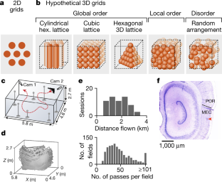
As animals navigate on a two-dimensional surface, neurons in the medial entorhinal cortex (MEC) known as grid cells are activated when the animal passes through multiple locations (firing fields) arranged in a hexagonal lattice that tiles the locomotion surface 1 . However, although our world is three-dimensional, it is unclear how the MEC represents 3D space 2 . Here we recorded from MEC cells in freely flying bats and identified several classes of spatial neurons, including 3D border cells, 3D head-direction cells, and neurons with multiple 3D firing fields. Many of these multifield neurons were 3D grid cells, whose neighbouring fields were separated by a characteristic distance—forming a local order—but lacked any global lattice arrangement of the fields. Thus, whereas 2D grid cells form a global lattice—characterized by both local and global order—3D grid cells exhibited only local order, creating a locally ordered metric for space. We modelled grid cells as emerging from pairwise interactions between fields, which yielded a hexagonal lattice in 2D and local order in 3D, thereby describing both 2D and 3D grid cells using one unifying model. Together, these data and model illuminate the fundamental differences and similarities between neural codes for 3D and 2D space in the mammalian brain.

This is a preview of subscription content, access via your institution

Access options

Access Nature and 54 other Nature Portfolio journals

Get Nature+, our best-value online-access subscription

24,99 € / 30 days

cancel any time

Subscribe to this journal

Receive 51 print issues and online access

185,98 € per year

only 3,65 € per issue

Buy this article

• Purchase on Springer Link
• Instant access to full article PDF

Prices may be subject to local taxes which are calculated during checkout

Similar content being viewed by others

Irregular distribution of grid cell firing fields in rats exploring a 3D volumetric space

Roddy M. Grieves, Selim Jedidi-Ayoub, … Kate J. Jeffery

The grid code for ordered experience

Jon W. Rueckemann, Marielena Sosa, … Elizabeth A. Buffalo

Entorhinal velocity signals reflect environmental geometry

Robert G. K. Munn, Caitlin S. Mallory, … Lisa M. Giocomo

Data availability

The data generated and analysed in the current study are available from the corresponding author on reasonable request.  Source data are provided with this paper.

Code availability

The code generated for the current study is available from the corresponding author on reasonable request.

Hafting, T., Fyhn, M., Molden, S., Moser, M.-B. & Moser, E. I. Microstructure of a spatial map in the entorhinal cortex. Nature 436 , 801–806 (2005).

Article   ADS   CAS   PubMed   Google Scholar  

Finkelstein, A., Las, L. & Ulanovsky, N. 3-D maps and compasses in the brain. Annu. Rev. Neurosci . 39 , 171–196 (2016).

Article   CAS   PubMed   Google Scholar  

Krupic, J., Burgess, N. & O’Keefe, J. Neural representations of location composed of spatially periodic bands. Science 337 , 853–857 (2012).

Article   ADS   CAS   PubMed   PubMed Central   Google Scholar  

Stensola, T., Stensola, H., Moser, M.-B. & Moser, E. I. Shearing-induced asymmetry in entorhinal grid cells. Nature 518 , 207–212 (2015).

Hayman, R., Verriotis, M. A., Jovalekic, A., Fenton, A. A. & Jeffery, K. J. Anisotropic encoding of three-dimensional space by place cells and grid cells. Nat. Neurosci . 14 , 1182–1188 (2011).

Article   CAS   PubMed   PubMed Central   Google Scholar  

Hayman, R. M., Casali, G., Wilson, J. J. & Jeffery, K. J. Grid cells on steeply sloping terrain: evidence for planar rather than volumetric encoding. Front. Psychol . 6 , 925 (2015).

Article   PubMed   PubMed Central   Google Scholar  

Casali, G., Bush, D. & Jeffery, K. Altered neural odometry in the vertical dimension. Proc. Natl Acad. Sci. USA 116 , 4631–4636 (2019).

Article   PubMed   PubMed Central   CAS   Google Scholar  

Yartsev, M. M., Witter, M. P. & Ulanovsky, N. Grid cells without theta oscillations in the entorhinal cortex of bats. Nature 479 , 103–107 (2011).

Taube, J. S., Muller, R. U. & Ranck, J. B. Jr Head-direction cells recorded from the postsubiculum in freely moving rats. I. Description and quantitative analysis. J. Neurosci . 10 , 420–435 (1990).

Sargolini, F. et al. Conjunctive representation of position, direction, and velocity in entorhinal cortex. Science 312 , 758–762 (2006).

Finkelstein, A. et al. Three-dimensional head-direction coding in the bat brain. Nature 517 , 159–164 (2015).

Solstad, T., Boccara, C. N., Kropff, E., Moser, M.-B. & Moser, E. I. Representation of geometric borders in the entorhinal cortex. Science 322 , 1865–1868 (2008).

Savelli, F., Yoganarasimha, D. & Knierim, J. J. Influence of boundary removal on the spatial representations of the medial entorhinal cortex. Hippocampus 18 , 1270–1282 (2008).

Yartsev, M. M. & Ulanovsky, N. Representation of three-dimensional space in the hippocampus of flying bats. Science 340 , 367–372 (2013).

Hales, T. C. A proof of the Kepler conjecture. Ann. Math . 162 , 1065–1185 (2005).

Article   MathSciNet   MATH   Google Scholar  

Stella, F. & Treves, A. The self-organization of grid cells in 3D. eLife 4 , e05913 (2015).

Article   PubMed Central   Google Scholar  

Mathis, A., Stemmler, M. B. & Herz, A. V. M. Probable nature of higher-dimensional symmetries underlying mammalian grid-cell activity patterns. eLife 4 , e05979 (2015).

Horiuchi, T. K. & Moss, C. F. Grid cells in 3-D: reconciling data and models. Hippocampus 25 , 1489–1500 (2015).

Article   PubMed   Google Scholar  

Boccara, C. N. et al. Grid cells in pre- and parasubiculum. Nat. Neurosci . 13 , 987–994 (2010).

Krupic, J., Bauza, M., Burton, S. & O’Keefe, J. Local transformations of the hippocampal cognitive map. Science 359 , 1143–1146 (2018).

Boccara, C. N., Nardin, M., Stella, F., O’Neill, J. & Csicsvari, J. The entorhinal cognitive map is attracted to goals. Science 363 , 1443–1447 (2019).

Sanguinetti-Scheck, J. I. & Brecht, M. Home, head direction stability, and grid cell distortion. J. Neurophysiol . 123 , 1392–1406 (2020).

Krupic, J., Bauza, M., Burton, S., Lever, C. & O’Keefe, J. How environment geometry affects grid cell symmetry and what we can learn from it. Phil. Trans. R. Soc. Lond. B 369 , 20130188 (2013).

Article   Google Scholar  

Stensola, H. et al. The entorhinal grid map is discretized. Nature 492 , 72–78 (2012).

Kropff, E. & Treves, A. The emergence of grid cells: intelligent design or just adaptation? Hippocampus 18 , 1256–1269 (2008).

Burak, Y. & Fiete, I. R. Accurate path integration in continuous attractor network models of grid cells. PLoS Comput. Biol . 5 , e1000291 (2009).

Article   ADS   MathSciNet   PubMed   PubMed Central   CAS   Google Scholar  

McNaughton, B. L., Battaglia, F. P., Jensen, O., Moser, E. I. & Moser, M.-B. Path integration and the neural basis of the ‘cognitive map’. Nat. Rev. Neurosci . 7 , 663–678 (2006).

Fiete, I. R., Burak, Y. & Brookings, T. What grid cells convey about rat location. J. Neurosci . 28 , 6858–6871 (2008).

Mathis, A., Herz, A. V. M. & Stemmler, M. B. Resolution of nested neuronal representations can be exponential in the number of neurons. Phys. Rev. Lett . 109 , 018103 (2012).

Article   ADS   PubMed   CAS   Google Scholar  

Stemmler, M., Mathis, A. & Herz, A. V. M. Connecting multiple spatial scales to decode the population activity of grid cells. Sci. Adv . 1 , e1500816 (2015).

Article   ADS   PubMed   PubMed Central   Google Scholar  

Sarel, A., Finkelstein, A., Las, L. & Ulanovsky, N. Vectorial representation of spatial goals in the hippocampus of bats. Science 355 , 176–180 (2017).

Omer, D. B., Maimon, S. R., Las, L. & Ulanovsky, N. Social place-cells in the bat hippocampus. Science 359 , 218–224 (2018).

Ulanovsky, N. & Moss, C. F. Hippocampal cellular and network activity in freely moving echolocating bats. Nat. Neurosci . 10 , 224–233 (2007).

Yovel, Y., Falk, B., Moss, C. F. & Ulanovsky, N. Optimal localization by pointing off axis. Science 327 , 701–704 (2010).

Skaggs, W. E., McNaughton, B. L., Wilson, M. A. & Barnes, C. A. Theta phase precession in hippocampal neuronal populations and the compression of temporal sequences. Hippocampus 6 , 149–172 (1996).

Henriksen, E. J. et al. Spatial representation along the proximodistal axis of CA1. Neuron 68 , 127–137 (2010).

Stukowski, A. Visualization and analysis of atomistic simulation data with OVITO—the Open Visualization Tool. Model. Simul. Mater. Sci. Eng . 18 , 015012 (2010).

Article   ADS   Google Scholar  

Larsen, P. M., Schmidt, S. & Schiøtz, J. Robust structural identification via polyhedral template matching. Model. Simul. Mater. Sci. Eng . 24 , 055007 (2016).

Article   ADS   CAS   Google Scholar  

Brandon, M. P. et al. Reduction of theta rhythm dissociates grid cell spatial periodicity from directional tuning. Science 332 , 595–599 (2011).

Koenig, J., Linder, A. N., Leutgeb, J. K. & Leutgeb, S. The spatial periodicity of grid cells is not sustained during reduced theta oscillations. Science 332 , 592–595 (2011).

Hansen, J.-P. & Verlet, L. Phase transitions of the Lennard-Jones system. Phys. Rev . 184 , 151–161 (1969).

Langston, R. F. et al. Development of the spatial representation system in the rat. Science 328 , 1576–1580 (2010).

Wills, T. J., Cacucci, F., Burgess, N. & O’Keefe, J. Development of the hippocampal cognitive map in preweanling rats. Science 328 , 1573–1576 (2010).

Eliav, T. et al. Nonoscillatory phase coding and synchronization in the bat hippocampal formation. Cell 175 , 1119–1130 (2018).

Derdikman, D. et al. Fragmentation of grid cell maps in a multicompartment environment. Nat. Neurosci . 12 , 1325–1332 (2009).

Torquato, S. & Stillinger, F. H. Jammed hard-particle packings: from Kepler to Bernal and beyond. Rev. Mod. Phys . 82 , 2633 (2010).

D’Albis, T. & Kempter, R. A single-cell spiking model for the origin of grid-cell patterns. PLoS Comput. Biol . 13 , e1005782 (2017).

Article   ADS   PubMed   PubMed Central   CAS   Google Scholar  

Monsalve-Mercado, M. M. & Leibold, C. Hippocampal spike-timing correlations lead to hexagonal grid fields. Phys. Rev. Lett . 119 , 038101 (2017).

Article   ADS   MathSciNet   PubMed   Google Scholar  

Weber, S. N. & Sprekeler, H. Learning place cells, grid cells and invariances with excitatory and inhibitory plasticity. eLife 7 , e34560 (2018).

Yoon, K. et al. Specific evidence of low-dimensional continuous attractor dynamics in grid cells. Nat. Neurosci . 16 , 1077–1084 (2013).

Guanella, A., Kiper, D. & Verschure, P. A model of grid cells based on a twisted torus topology. Int. J. Neural Syst . 17 , 231–240 (2007).

Fuhs, M. C. & Touretzky, D. S. A spin glass model of path integration in rat medial entorhinal cortex. J. Neurosci . 26 , 4266–4276 (2006).

Klukas, M., Lewis, M. & Fiete, I. Efficient and flexible representation of higher-dimensional cognitive variables with grid cells. PLoS Comput. Biol . 16 , e1007796 (2020).

Burak, Y. & Fiete, I. Do we understand the emergent dynamics of grid cell activity? J. Neurosci . 26 , 9352–9354 (2006).

Rowland, D. C., Roudi, Y., Moser, M.-B. & Moser, E. I. Ten years of grid cells. Annu. Rev. Neurosci . 39 , 19–40 (2016).

Download references

Acknowledgements

We thank A. Treves for extensive discussions, A. V. M. Herz and E. Katzav for helpful suggestions; F. Stella, E. D. Karpas, T. Tamir, A. Rubin, A. Finkelstein, S. R. Maimon, S. Ray, D. Omer, S. Palgi and A. Sarel for comments on the manuscript; J.-M. Fellous for contributing to the initial stages of this project; S. Kaufman, O. Gobi and I. Shulman for bat training; A. Tuval for veterinary support; C. Ra’anan and R. Eilam for histology; M. P. Witter for advice on histological delineation of MEC borders; B. Pasmantirer and G. Ankaoua for mechanical designs; and G. Brodsky and N. David for graphics. We thank the Methods in Computational Neuroscience course at MBL, Woods Hole, where the modelling work was initiated. N.U. is the incumbent of the Barbara and Morris Levinson Professorial Chair in Brain Research. Y.B. is the incumbent of the William N. Skirball Chair in Neurophysics. This study was supported by research grants to N.U. from the European Research Council (ERC-CoG – NATURAL_BAT_NAV), Israel Science Foundation (ISF 1319/13), and Minerva Foundation, and by the André Deloro Prize for Scientific Research and the Kimmel Award for Innovative Investigation to N.U. Y.B. acknowledges support from the Israel Science Foundation (ISF 1745/18), the European Research Council (ERC-SyG – KiloNeurons), and the Gatsby Charitable Foundation. H.S. acknowledges support from the Gatsby Charitable Foundation.

Author information

Authors and affiliations.

Department of Neurobiology, Weizmann Institute of Science, Rehovot, Israel

Gily Ginosar, Johnatan Aljadeff, Liora Las & Nachum Ulanovsky

Department of Bioengineering, Imperial College London, London, UK

Johnatan Aljadeff

The Edmond and Lily Safra Center for Brain Sciences, The Hebrew University of Jerusalem, Jerusalem, Israel

Yoram Burak & Haim Sompolinsky

Racah Institute of Physics, The Hebrew University of Jerusalem, Jerusalem, Israel

Center for Brain Science, Harvard University, Cambridge, MA, USA

Haim Sompolinsky

You can also search for this author in PubMed   Google Scholar

Contributions

G.G, L.L. and N.U. conceived and designed the experiments. G.G. conducted the experiments, with contributions from L.L. G.G. analysed the experimental data. L.L. and N.U. guided the data analysis. J.A., Y.B. and H.S. conducted the theoretical modelling, and J.A. analysed the model results. G.G. and N.U. wrote the first draft of the manuscript, with major input from L.L. All authors participated in writing and editing of the manuscript. N.U. supervised the project.

Corresponding author

Correspondence to Nachum Ulanovsky .

Ethics declarations

Competing interests.

The authors declare no competing interests.

Additional information

Peer review information Nature thanks Mark Brandon, Torkel Hafting and the other, anonymous, reviewer(s) for their contribution to the peer review of this work.

Publisher’s note Springer Nature remains neutral with regard to jurisdictional claims in published maps and institutional affiliations.

Extended data figures and tables

Extended data fig. 1 expected properties of 3d grid cells, and coverage of 3d space by the bats’ behaviour..

a , Five basic properties of 2D grid cells. b , Expected properties of 3D grids under five hypothetical possibilities, ranging from highly ordered to random arrangement of fields. c , d , Bat behaviour covers 3D space. c , Examples of bat trajectories in the flight room. Rows: one example session from each of the four bats included in this study. Columns show different viewing perspectives: 3D view; top view of the room ( xy ); and side views of the room ( xz and yz ). Note that for bat 4 only, part of the room (grey area) was blocked off by a see-through nylon mesh (see  Methods ). d , Histograms of distance flown per session, plotted separately for each of the four bats; we included here only sessions in which we recorded at least one of the 125 well-isolated neurons that passed the inclusion criteria for analysis.

Extended Data Fig. 2 A series of histological sections from one bat, showing two tetrode tracks in MEC layer 5.

Two tetrode tracks that enter from postrhinal cortex (POR) and progress along layer 5 of MEC in bat 2. Four sagittal Nissl-stained sections are arranged from medial (top) to lateral (bottom). Left, wide view (scale bar, 1,000 μm); right, zoom-in onto the region of the tetrode tracks (scale bar, 500 μm). The postrhinal (dorsal) border of MEC is marked by a black line. The combination of the angled tetrode penetration (see  Methods ) and the sagittal slicing of the brain resulted in tetrode tracks that are recognizable as a small hole (sometimes surrounded by glial scar) that proceeds over many consecutive sections. The distance of the hole (track) from the postrhinal border of MEC is indicated on the right. Coloured circles mark the tracks of the two tetrodes (purple, tetrode 1 (TT1); green, tetrode 4 (TT4)). The lesion at the end of the track of tetrode 1 (purple) is visible in section 31c (section numbers are indicated). The lesion at the end of the track of tetrode 4 (green) is visible in section 29b.

Extended Data Fig. 3 Firing fields, and additional examples of cells.

a , Peak detection: firing-rate map of an example cell, with overlaid black dots marking the positions of the detected field peaks (see  Methods ). Note that only the peaks of the visible fields are displayed here (not plotting the peaks for fields ‘buried’ deep inside the 3D volume of the map). b , Threshold for peak detection shuffle (one of three criteria for a field to be valid; these three criteria narrowed the n  = 125 cells to n  = 78 cells): an identified peak was included in the analysis if the firing rate in its peak voxel was higher than the firing rate in the same voxel in 75% of the spike shuffles (see  Methods ). Shown are the shuffle percentiles for all fields (both above and below this threshold); the 75% threshold was set at a natural kink in the distribution. c , Number of fields per neuron: a histogram for all the neurons with valid fields ( n  = 78 cells), showing the number of fields per cell. A threshold of 10 fields was set for a neuron to be considered as ‘multifield’ ( n  = 66 cells, black bars; grey bars show cells below the threshold); see  Methods for the rationale of setting this 10-field threshold. Example cells with varying numbers of fields are shown in d . d , Examples of cells with varying numbers of fields, including <10 fields (two left cells, not considered as multifield cells), and both grid and non-grid multifield cells with ≥10 fields. Plotted as in Fig. 2a, b . Top: 3D firing-rate maps. Bottom: box plots showing the median field sizes in the x , y and z directions. Horizontal line, median; box limits, 25th to 75th percentiles; whiskers,10th to 90th percentiles. Shown are the results of Wilcoxon rank-sum tests comparing field dimensions in x vs. y , y vs. z and x vs. z , Bonferroni-corrected for three pairwise comparisons; n.s., non-significant; the number of fields for each cell (that is, the n for each test) is written above each firing-rate map. e , Two example neurons with significant field elongations; plotted as in d (overall, 9 out of 66 neurons showed significant field elongations). Note that these two neurons differed in their elongation direction. Wilcoxon rank-sum test comparing field dimensions in x vs. y , y vs. z and x vs. z , Bonferroni-corrected for three pairwise comparisons: left cell: P yz  = 0.03, P xz  = 0.003; right cell: P xy  = 0.006 (Bonferroni-corrected for three comparisons); the number of fields for each cell (that is, the n for each test) is written above each firing-rate map. In the 9 cells with significant field elongation, fields did not resemble columns and elongation was weak and not systematic, that is, the elongation direction was heterogeneous and differed across these 9 elongated neurons.

Extended Data Fig. 4 Non-stereotypy of flights, and diversity of passes through fields: part I.

a , Passes per field: histograms showing the number of flight passes creating each firing field (passes per field and passes with spikes per field serve as two of three criteria for a detected field to be considered valid). The four histograms correspond to all passes within the fields (top) and all passes with spikes within the field (bottom), computed for two different values of the radius from the field’s peak: 30 cm (left) and 50 cm (right). b , Flight non-stereotypy: a histogram showing the percentage of flights of each cell that passed through the same sequence of fields, within two different values of the distance (radius) from the field’s peak: 30 cm (left) and 50 cm (right). Flights that pass through the same sequence of fields correspond to a stereotypic trajectory of the bat: for example, if the same flight sequence repeats four times, it would appear here in the fourth bin, that is, with a value of 4 for ‘No. of flights with same sequence’. The results here show that most flights are in fact unique and do not repeat more than once for the same cell (see large bin with value 1 for ‘No. of flights with same sequence’), which suggests that the bats’ flights were non-stereotypic. c , The xy projections of the trajectories that passed through 20 example fields. Shown are trajectories within a 0.5-m radius around the field’s peak (this is the typical radius of grid fields in our data). We extracted the trajectories for all the 1,113 fields of the 66 multifield neurons, as follows: for each field we took a 3D sphere with 0.5-m radius around the field’s peak, then extracted the 3D trajectories through this field, and then projected these 3D trajectories onto xy (2D projections). The Rayleigh vector length (RV) of the xy -projected trajectories was then computed for each field. Here we plotted one example field from approximately every fifth percentile of the RV distribution—a total of 20 example fields, ordered from low to high RV. The RV value and percentile (in parentheses) are indicated: top left example is from the first percentile of the RV = lowest RV (most isotropic trajectories); bottom right example is from the 99th percentile of the RV = highest RV (most uni-directional trajectories). Scale bar, 0.5 m. d , The RV distribution across all the fields ( n  = 1,113), calculated on the trajectories forming each field (see examples in c ). Median RV of this distribution = 0.25: this is a relatively low value, indicating rather isotropic flights through most fields.

Extended Data Fig. 5 Non-stereotypy of flights, and diversity of passes through fields: part II.

a , Two examples of individual cells (columns), depicting the firing rates in each of the fields based on the trajectories coming from specific take-off balls (top matrices) or specific landing balls (bottom matrices); colour-coded from 0 (blue) to maximum firing rate (red; value indicated). In each matrix, the variety of firing rates in each row of the matrix (corresponding to each field) shows that the firing of each field was created by trajectories originating from a variety of take-off balls and ending on a variety of landing balls. b , Percentage of fields per cell that are created from diverse trajectories. Box plots show the percentages of fields per cell whose behavioural trajectories involved at least 50% of the take-off balls (left) or landing balls (right). This analysis was done for the three bats for which we used landing balls. Horizontal line, median; box limits, 25th to 75th percentiles; whiskers,10th to 90th percentiles. The high percentage shown here means that across cells, the large majority of fields per neuron involved most of the take-off balls and landing balls—that is, the bats’ flights were diverse and non-stereotypic. c , Histograms showing the number of fields that were formed by trajectories that originated from various numbers of different take-off balls (top) and ending at various numbers of different landing balls (bottom). This analysis was done for the three bats for which we used landing-balls. d – f , As in a – c , but here instead of take-off and landing balls we examined the firing-rate at different directions of the trajectories passing through the field. This analysis was done on all the four bats. d , Examples of two individual cells. e , Percentage of fields in which the trajectories with spikes that occurred close to the field-peak (within 50 cm of the field peak) came from ≥50% of the direction bins. f , Distribution of the percentage of direction bins for trajectories with spikes that passed through each field. For example, 60% on the x -axis means that the spikes of that field came from 60% of all the possible direction bins; that is, the flight trajectories with spikes that passed through that field spanned 60% of all the possible direction bins (60% of 360°; we used here 36° bins)—a high diversity of directions.

Extended Data Fig. 6 Searching for global and local order.

a , Two lattices were proposed as theoretically probable structures of 3D grids 16 , 17 : these lattices exhibit a hexagonal arrangement of spheres, and were proved to be the optimal arrangement for densest sphere packing in infinite 3D space 15 . These lattice arrangements—face centred cubic (FCC) and hexagonal close pack (HCP)—are widely found in chemistry. Both of these lattices are comprised of layers of spheres arranged in a hexagonal pattern (denoted here as layers A, B and C); the two lattices differ in the phase of these layers. Each layer is placed in one of two optional sets of holes created by the lower layer: the HCP lattice has an A–B–A pattern of layers (left); the FCC lattice has an A–B–C pattern of layers (right). b , Illustration of the procedure of fitting data to hexagonal lattices (see  Methods ). Cartoon in 2D depicts the fitting that we used in 3D to fit the recorded 3D field arrangements to perfect FCC and HCP lattices. To find the best-fitting lattice for each of our recorded cells, we compared each cell with 3 million variations of FCC and HCP perfect lattices; this was done separately for FCC and HCP lattices (1.5 million variations for FCC and 1.5 million for HCP). In each iteration, we found for each of the recorded fields (purple spheres) the closest field in the perfect lattice (the simulated perfect lattice fields are depicted by dotted blue circles; red lines depict the distances between a recorded field and its nearest simulated lattice field). We then computed the squared distance from each recorded field to its closest simulated synthetic field; we summed these squared distances and computed the root, to yield the root mean square (RMS) error of each cell for each of the 1.5 million FCCs or 1.5 million HCPs. The cell’s lowest RMS error across all the 1.5 million FCC lattices was termed the ‘FCC fit error’, and was then compared to the FCC fit errors that were analogously computed for all the shuffles (that is, for each shuffle we found the minimal FCC fit error over the 1.5 million synthetic FCC’s). The same was done for HCP. c , Distribution of local angles. There was no angle-bias of local 3D angles, suggesting no local orientational (angular) order in the field arrangements. Top, local angles were computed between triplets of nearest-neighbouring fields; to avoid edge effects, we computed the angles only for fields that were within the convex hull of field arrangement. Grey, all recorded multifield cells; black line, shuffled data (using spike shuffling). Middle and bottom, distributions of local angles plotted separately for 3D grid cells (middle: red) and non-grid multifield cells (bottom: blue), together with shuffle data (black lines). The distributions for recorded cells did not differ significantly from the spike-shuffled data (black; indicated are the P values of Kolmogorov–Smirnov tests between data and shuffles). d , e , The calculation of the CV of distances to nearest neighbouring fields. d , Cartoon illustrating the three distances between each field and its three nearest neighbouring fields. These distances were then pooled across all fields (while avoiding double-counts), and the CV over these distances was calculated to quantify how fixed is the distance scale of the neuron (see  Methods ). e , Rationale for why the CV was computed over three nearest neighbours, and not 1, 2 or >3 nearest neighbours. Right, a perfect 2D lattice arrangement will yield low CV values regardless of how many nearest neighbours are considered: three (bottom) or two (top). Left, a periodic 1D structure (‘fields along a string’)—which is not a 2D lattice—may still yield a low CV when considering only two neighbours (top left), but a high CV when considering three or more nearest neighbours (bottom left). Thus, three is the minimal number of nearest neighbours that can differentiate these possibilities, and unequivocally characterize the 3D arrangement of fields. We did not use more than three neighbours, because using a large number of neighbours may accentuate possible edge effects. f , Comparison of the CV measure and gridness score for cells in 2D. Left, scatter plot of the CV of nearest-neighbour distances versus the classical 2D gridness score, for medial entorhinal cortex neurons recorded in rats running in 2D in the Moser laboratory (courtesy of M.-B. Moser and E. I. Moser, from https://www.ntnu.edu/kavli/research/grid-cell-data ; n  = 259 cells; we excluded from analysis putative interneurons (mean firing rate >5 Hz), non-spatial neurons (cells with spatial information <0.2 bits per spike) and border cells (manually excluded)). The Pearson correlation of this scatter and its P value are given in the top-right corner. Right, example firing-rate maps of two cells. Top, a spatial non-grid cell with low gridness score and high CV; bottom, a grid cell with high gridness score and low CV. The locations of these two cells on the scatter plot are indicated. Here the gridness score was computed as described in the Methods, and the CV was computed using the distances of the two nearest neighbours of each field, rather than three nearest neighbours as done for 3D cells, because in 2D many cells did not have enough fields. g , h , The lack of global order could not be explained by proximity to room borders. g , Local angles throughout the room: shown is a scatter plot of the local angles between triplets of neighbouring fields as a function of their distance from the nearest wall. Points were slightly jittered in the x -axis, for display purposes only. Pearson correlation and significance are shown. The non-significant correlation suggests that the walls did not affect the 3D arrangement of fields. h , CV of nearest-neighbour distances throughout the room: shown is a histogram of the differences between CVs of fields at the edges of the room and the CVs of fields in the centre of the room (CV edges  − CV centre ). The border between ‘centre’ and ‘edges’ of the room was defined as the median distance of all the fields from their closest wall. Grey bars, histogram for all multifield cells ( n  = 66 cells); black line, histogram for shuffles done per neuron, using spike shuffling. P value of Kolmogorov–Smirnov test of data versus shuffles is indicated. The non-significant difference suggests that the walls did not affect the 3D arrangement of fields.

Extended Data Fig. 7 The firing of 3D grid cells and non-grid multifield cells cannot be explained via a global lattice that undergoes distortions (scaling, shearing, or barrelling).

a – c , Mean CVs of distances between neighbouring fields, calculated after un-distorting the field positions of multifield cells ( n  = 66); shown separately for each individual bat (columns 1–4), and for all the cells from all bats pooled together (column 5). We did three types of un-distortion: un-scaling, un-shearing, and un-barrelling (see  Methods ). a , Un-scaling: field positions were scaled by a factor α along the specified axis. α  < 1 corresponds to shrinking towards the middle of the room along the specified axis, α  > 1 means expansion, α  = 1 corresponds to no change. The three rows correspond to un-scaling along three pairs of axes: xy , yz , and xz . Each heat-map describes the mean CV for all possible combinations of un-scaling of two axes: α 1 describes the first axis (in xy (first row) it corresponds to x ), and α 2 describes the second axis (in xy it corresponds to y ). CV is colour-coded from minimal value (blue) to maximal value (red), and these values are written above each matrix. White squares indicate no scaling ( α 1  =  α 2  = 1, that is, original data). b , Un-shearing: the fields of each cell underwent shearing/un-shearing as described 4  (see  Methods ), where shearing was done by two walls simultaneously (yielding 15 possible combinations of shearing, all shown here (rows)); we computed the two possible shearing directions (positive and negative γ -factor, which can also be thought of as shearing and un-shearing). The writing on the left indicates the two walls that create the shearing and the axes in which the shearing is occurring (for example, xz shear x means that the xz wall is creating a shearing along the x -axis). Factor γ 1 corresponds to the first line (for example, xz shear x in the top row), and γ 2 corresponds to the second line (for example, yz shear y in the top row). Heat-map shows mean values of CV, colour-coded from minimum (blue) to maximum (red; values indicated above the panel). White squares indicate no shearing ( γ 1  =  γ 2  = 0, that is, original data). c , Un-barrelling: a barrelling transformation (also known as fisheye lens distortion) and un-barrelling transformation (also known as pin-cushion distortion) was performed on the field arrangement of each cell. Plots show mean CV values as a function of the barrel and un-barrel factor β , for the different 2D planes along which the barrelling/un-barrelling was done ( xy , yz , xz (rows)). All the transformations in a – c (scaling, shearing, barrelling) showed that distorting or un-distorting away from the original field arrangement increases the CV—which argues against the notion that the original field arrangements constitute a global lattice that underwent distortions.

Extended Data Fig. 8 Both 3D grid cells and non-grid multifield cells exhibit an anatomical gradient along the dorsoventral axis of MEC, as seen in rodent 2D grid cells.

a , Examples of recording sites and firing-rate maps of cells along the inter-field distance gradient, here using the spike-shuffling method as in Fig. 3b . Central scatterplot: both 3D grid cells (red) and non-grid multifield cells (blue) exhibited an increase in inter-field distance as a function of the recording depth along the dorsoventral axis of MEC—akin to what is known from rodent 2D grid cells 1 . 3D grid cells were identified using spike shuffling; data points were pooled here across tetrodes and bats, and include only cells with high-quality histology that allowed precise assessment of recording depth within MEC ( n = 8 grid cells, n = 28 non-grid multifield cells). Side panels: two histology examples, and their associated 3D firing-rate maps. Left, 3D grid cell recorded in layer 3; right, non-grid multifield cell recorded in layer 5. b , The increase in inter-field distance along the dorsoventral axis of MEC is also evident in individual tetrode tracks (TT). Shown are examples of three tetrode tracks, which proceeded mostly along a single cortical layer (indicated). Pearson correlation coefficients and their P values are indicated. c , Dorsoventral gradient, plotted as in Fig. 3b , but here classifying grid cells based on the field-shuffling method (rather than the spike-shuffling method as in Fig. 3b ). We identified 20 neurons as 3D grid cells using field shuffling; included in these scatter-plots were only cells with high-quality histology that allowed precise assessment of recording depth within MEC ( n = 11 grid cells, n = 25 non-grid multifield cells). Left, gradient of inter-field distances between neighbouring fields as a function of recording depth in MEC (distance from the postrhinal border of MEC); right, gradient of number of fields per cell as a function of recording depth. Note that the gradient is exhibited by both 3D grid cells (red) and non-grid multifield cells (blue), suggesting they are not two separate populations of neurons, but a continuum. Shown are Pearson correlation coefficients and their P values.

Extended Data Fig. 9 Border cells and firing characteristics of the various cell classes.

a – c , Border cells. a , Definition of border cells in 3D arenas. We considered only neurons for which a 2D firing field was detected in each of the cell’s 2D planes (see  Methods ). 2D firing-rate maps were plotted in the three principal 2D views of the room geometry: the top view xy , and the two side views xz and yz (green, orange and blue, respectively). We defined an elongation index for each field in each 2D plane as the field size along the more elongated axis/field size along the less elongated axis; the elongation index was computed separately for all three 2D planes ( xy , xz , yz ). A border field was defined as a field that was significantly elongated in exactly two out of the three views (for determining the significance we used the elongation index for each field and compared it to the elongation indices of spike shuffles; 99% criterion). Significant 1D border cells (left) were defined as ‘sausage-shaped’ neurons in which: (i) two of the 2D planes (2D views) exhibited firing fields with an elongation index > 2, which was also significantly higher than shuffled data (>99% of the shuffles); and (ii) the third plane (2D view) exhibited a firing field that was non-elongated, and was smaller than in the two elongated planes (left, blue square), thus defining a 1D ‘sausage’. Significant 2D planar border cells (right) were defined as ‘pancake-shaped’ neurons in which: (i) two of the 2D planes (2D views) exhibited firing fields with elongation index >2, which was also significantly higher than shuffled data (>99% of the shuffles); and (ii) the third plane (2D view) exhibited a firing field that was non-elongated, and was larger than in the two elongated planes (right, green square), thus defining a 2D ‘pancake’. b , c , A full depiction of the example border cells plotted in Fig. 4b , here shown also with trajectories and spikes, as well as an additional example. b , Example of a border cell that exhibited firing along a 1D border of space—in this case, along the wall edge. Left, a top view of the room ( xy ); middle, right, side views ( xz and yz ). Top, flight trajectory (grey) with spikes superimposed (red dots); bottom, firing rate maps, colour-coded from zero (blue) to the maximal firing rate across the three views of each cell (red). White line, edges of the detected firing field (enlarged by one bin for display purposes); indicated are the peak firing-rate and elongation index (EI; see  Methods ). Grey rectangle, area of the room that was made inaccessible for one of the four bats (see  Methods ). c , Examples of border cells that exhibited firing along a 2D planar border of space—in this case, the floor. Plotted as in b . Top cell also shown in Fig. 4b . d , e , Characteristics of the various cell classes. d , Firing characteristics for the different functional cell classes in MEC during 3D flight (mean ± s.d. across cells; the column of head-direction cells is based on significant azimuthal head-direction cells). Peak firing rate (FR): the highest firing rate in the 3D firing rate map. Mean firing rate: the mean of the 3D firing rate map (second row) and the ratio of total spikes in flight/total time in flight (third row); these values were very similar because the 3D behaviour was quite uniform. Fourth row: Theta index 8 , 19 , 39 , 40 (TI) computed as in ref. 19 , where a criterion of TI > 5 was used as threshold for defining theta-modulated cells. All the cells in our study, including all the grid cells, exhibited TI < 5, indicating a lack of theta rhythmicity in the MEC of flying bats, consistent with previous findings on bat MEC cells in 2D 8 , 44 . e , Examples of spike-train autocorrelations (top) and their power spectra (bottom) for the various cell classes. The theta index is indicated above the power spectra. Note that for the four grid cells, the two leftmost examples have theta index below the population mean (see d ), whereas the two rightmost examples have theta index above the population mean; none of these four examples exhibited clear oscillations.

Extended Data Fig. 10 Distribution of best-fitting temperatures in the Lennard–Jones pairwise interactions model, and comparison to alternative pairwise-interactions models.

a – c , Simulations of highly structured cells with low CV (CV < 0.25, n  = 29 neurons). a , Distribution of the best-fitting temperatures ( T ) in the Lennard–Jones (LJ) pairwise interactions model (red, 3D grid cells identified by spike shuffling; blue, non-grid multifield cells). The best-fitting temperature for the model (log 10 T  = 0.5; black dashed line) was computed as the average logarithm of the temperatures across all these cells; this temperature was consistent with the individual temperatures for almost all of the cells. The small variation in the fitted temperatures allowed us to use a single temperature for all the cells (log 10 T  = 0.5, dashed line). b , c , Comparison of multiple models of short-range repulsion and long-range attraction (Lennard–Jones, modified Lennard–Jones, and difference-of-Gaussians (DOG) potentials). b , Quantifying the match between model and data. Three rightmost bars: distances between the RDF of the data and the RDFs of the pairwise interactions models: Lennard–Jones, modified Lennard–Jones, and DOG (log 10 T  = 0.5 for all models). Left bar, distance between the RDF of the data and the RDF of the random Poisson model (in which the fields were randomly distributed in the 3D region visited by the bat). N  = 1,000 simulated RDFs for each model; shown mean ± s.e.m. The distance between the RDFs of the model simulations and the RDF of the data was substantially smaller for the three pairwise interactions models than for the random Poisson model ( t -test: P  < 10 −300 for all three comparisons). c , Best-fitting temperatures (in log scale, mean ± s.d.) for neurons with CV < 0.25, plotted for the three pairwise interactions models. All these potentials yielded similar best-fitting temperatures: the Lennard–Jones and modified Lennard–Jones potentials yielded very similar best-fitting temperatures, and the DOG potential yielded a slightly lower temperature. The vertical dashed line denotes the temperature that was used for the bulk of the simulations in this study with the Lennard–Jones potential (log 10 T  = 0.5). We note that for the modified Lennard–Jones and DOG potentials, the match between the RDF of the data and the RDF of the model was also very good for log 10 T  = 0.5 (see b , where for all three pairwise interactions models we used log 10 T  = 0.5). d , e , Simulations for high-CV cells (CV > 0.25, neurons not exhibiting an ordered arrangement of fields; n  = 37 neurons). d , Distribution of the best-fitting temperatures in the Lennard–Jones pairwise interactions model (red, 3D grid cells; blue, non-grid multifield cells). The average logarithm of the best-fitting temperatures across these neurons was ~ log 10 T  = 3.5 (black dashed line). e , Quantifying the match between model and data; t -test, P values indicated. Three rightmost bars: distances between the RDF of the data and the RDFs of the three pairwise interactions models (temperatures used here: Lennard–Jones, log 10 T  = 3.5; modified Lennard–Jones, log 10 T  = 1.5; DOG, log 10 T  = 1; these were the best-fitting temperatures for each of the models; note that these temperatures correspond to a much higher noise level than in the pairwise interactions models in a – c , where we considered neurons with CV < 0.25 and fitted a temperature of log 10 T  = 0.5). Left bar, distance between the RDF of the data and the RDF of the random Poisson model. N  = 1,000 simulated RDFs for each model; shown mean ± s.e.m.

Extended Data Fig. 11 Modelling: index definitions, 2D grids, and effective density.

a , Definition of the regularity index (RI), computed as the relative height of the maximum versus the minimum in the RDF (excluding its first peak); that is, the RI reflects the modulation depth of the second (or third) peak of the RDF (see  Methods ). b , Definition of effective density ρ eff , which is defined as r 0 /mean inter-field distance (see  Methods ). Note that when the fields are at their equilibrium position, at distances equalling the minimal energy of the Lennard–Jones potential, the effective density is ρ eff  = 0.9; that is, ρ eff  = 0.9 is the ‘natural’ effective density. c , Two examples of 2D simulated cells, showing field positions (bottom) and autocorrelograms (top, zoomed in on the centre). Numbers above autocorrelograms indicate the classical 2D gridness score ( g ). The left example is also shown in Fig. 5d . d , Distribution of gridness scores in all the pairwise-interaction 2D simulations (room size: 2 × 2 m). Many of the 2D simulations resulted in a high gridness score, indicating a highly ordered hexagonal organization. e , Plot of the classical 2D gridness score 8 , 10 , 19 versus 2D room size, for our 2D model simulations (simulations in a room of size a  ×  a  × 10-cm height; the gridness score was computed as described above (see  Methods ) and is shown as mean ± s.e.m.; minimum 500 simulations per room size a (the number of simulations varied because they were chosen post hoc to match the nominal ρ eff )). This plot is shown for fixed effective density ρ eff  = 0.9, which is the ‘natural’ value for ρ eff , where the local distances equal the minimal energy distance r min of the Lennard–Jones potential (see b ; note that ρ eff is defined as: ρ eff  =  r 0 / d NN , where d NN is the mean nearest neighbour distance (see  Methods ); because r min  =  r 0  × 1.12 in the Lennard–Jones function, this yields: ρ eff  = ( r min /1.12)/ d NN ≈ 0.9 ×  r min / d NN . That is, when d NN  =  r min , this yields ρ eff  = 0.9). In other words, ρ eff  = 0.9 is the effective density that yields inter-field distances that match the minimum of the Lennard–Jones potential. We note that this effective density is also well within the empirically measured range of effective densities for our experimental data (see f ). f , Distribution of effective density of fields ρ eff in our experimental data, computed using the best-fitted scale parameter r 0 for each neuron (shown here are the n = 29 multifield cells with CV < 0.25). g , Regularity index as a function of room height. Simulations were done in 10-cm increments of room height, going from effectively 2D arena (0.1 m ceiling) to a full 3D room (2.5 m ceiling), as in Fig. 5e . Each curve was computed for a fixed effective density ρ eff (see b ); different curve shading corresponds to different ρ eff values, from light to dark grey ( ρ eff  = 0.75 to ρ eff  = 1). Thick curve (shown in Fig. 5e ): ρ eff  = 0.9, a value within the range seen in our data (see f ), and which is the ‘natural’ effective density corresponding to the equilibrium positions of the fields (see b ). Left, computed for parameters corresponding to the 3D data, using r 0  = 1 m and a 5 × 5 m floor (with varying ceiling height). Right: computed for parameters corresponding to 2D data, using r 0  = 0.5 m and a 2 × 2 m floor (with varying ceiling height). Dashed line marks the value of r 0 used. Note the drop in regularity values when going from 2D to 3D; at this transition point the room height is slightly smaller than the distance parameter r 0 of the Lennard–Jones potential (and thus the room height allowed a second layer of fields).

Extended Data Fig. 12 3D grid cells are better explained by the pairwise interactions model than by jittered FCC or jittered HCP models; and pairwise interactions lead to a local but not global order at low temperatures of the model.

a , RDF plots for three models (top row, green: Lennard–Jones pairwise interactions model; middle and bottom rows, dark and light purple: jittered FCC and jittered HCP models, where the RDFs were computed for jittered FCC and jittered HCP models with the same nearest-neighbour mean distance ( d NN ) and CV of distances ( CV NN ) as used in the pairwise interactions model). Each model was simulated using three temperatures ( T ) of the model (left, zero temperature T  = 0, a non-biological scenario with no noise; middle, low temperature (log 10 T  = −1) with little noise; right, the higher temperature that fitted well our experimental 3D data (log 10 T  = 0.5)). For the temperature fitted to the data (log 10 T  = 0.5), note the comparison of the RDF for the pairwise interactions model (top right, green) to the RDF for a random Poisson model (grey): the peak of the RDF is much sharper around r  = 1 in the pairwise interactions model (green), indicating preserved local distances between nearby fields. Note that for very low temperatures with little or no jitter (left, middle), the jittered FCC and jittered HCP models showed very repetitive and distinct peaks in the RDF as a function of distance r , indicating a near-perfect lattice—as expected from FCC and HCP with no jitter ( T  = 0) or very small jitter (low temperature log 10 T  = −1). By contrast, for the pairwise interactions model, at low temperatures (both at log 10 T  = −1 and T  = 0) the RDF was non-zero at all distances (see insets), which is not consistent with a perfect global lattice. At T  = 0, the RDF seems more consistent with a distorted FCC lattice, but with preserved local distances. In other words, even at very low temperatures, the pairwise interactions model exhibited local distances without a global lattice. b , Distributions of local angles for the different models, following the same organization as a . Even at T  = 0, the pairwise interactions model yielded field arrangements with a continuous angle distribution, with all possible angles (except very small angles that cannot occur for nearest-neighbour triangles)—in contrast to the jittered FCC and jittered HCP arrangements where angles concentrated solely in discrete values, which indicates again that even at T  = 0, the pairwise interactions model does not exhibit a perfect global lattice. Here again, at the temperature fitted to the 3D data (log 10 T  = 0.5), the pairwise interactions model yielded a more ordered arrangement than the random Poisson (top right, green curve for Lennard–Jones: see the mild peak at an angle of 60°, as compared to the grey curve for random Poisson: no peak). This means that the pairwise interactions model yielded stronger local orientational order than randomly arranged fields. c , d , Energy convergence of the Lennard–Jones pairwise interactions model at the temperature that best fitted the 3D data (log 10 T  = 0.5, orange) and at T  = 0 (light blue). c , Energy per pair of fields versus the step number of the simulation. d , Left, energy change versus the step number of the simulation, plotted in linear–log scale for both temperatures. Right, energy change of the simulations for T  = 0, plotted in log–log scale. Shading in c , d depicts s.e.m. Note that c , d show that for the temperature which was used to fit our model to the data (log 10 T  = 0.5, orange), the system converged to an asymptote very rapidly, long before we finished running the simulations—that is, the system rapidly reached equilibrium; therefore, the simulations reported in this study correspond to a system in equilibrium.

Extended Data Fig. 13 Comparing the pairwise interactions model for 3D versus 2D, for six combinations of model parameters T and r 0 (varying the number of fields).

a – f , Regularity phase planes for 2D and 3D (see Extended Data Fig. 11a for illustration of the regularity index)—plotted as a function of room size, a , and number of fields, N . Room dimensions: 2D, a  ×  a  × 10-cm height; 3D, room-size a  ×  a  ×  a /2. The three rows ( a , b and c , d and e , f ) correspond to a changing temperature parameter T ( c , d show the temperature that was best fitted to the experimental data: log 10 T  = 0.5). The two columns ( a , c , e and b , d , f ) correspond to a changing distance parameter r 0 of the Lennard–Jones potential (values of T and r 0 are indicated). For each panel, we compared simulations in 2D (left) and in 3D (right). The top graphs in each panel show the regularity index (grey scale) for various combinations of a and N (we conducted simulations for N  ≥ 10, corresponding to multifield cells, which have ≥10 fields). Note that all these simulations exhibited much higher regularity of field arrangements in 2D than in 3D. Red hatched area denotes a non-plausible region, where the experimentally observed field diameters (~20 cm for published 2D rat grid cells 24 and ~1 m in our 3D bat grid cells) do not allow fitting N such fields into a room of size a (see  Methods ). The bottom graphs show the RDF as a function of r (normalized distance) for two specific values of a , N (marked by small squares in the top graphs). Left, 2D simulation for a  = 2 m, N  = 30 fields (the approximate arena size and number of fields for a typical rat 2D grid cell from dorsal MEC 24 ); right, 3D simulation for a  = 5 m, N  = 20 fields (corresponding to our typical 3D data from bats). RDFs plotted as in Fig. 5d . Note that for all six parameter combinations ( T , r 0 ; a – f ), the 2D simulations showed a high regularity index (owing to a prominent second peak emerging in the RDF in 2D) for a large portion of the phase plane, and in particular in the a , N combination corresponding to a typical 2D grid cell from rat dorsal-MEC 24 (black pixel in the left panels)—whereas all 3D simulations showed a low regularity index for a , N corresponding to our data (white pixel in the right panels). A similar difference between 2D and 3D was also found when plotting phase planes of room size a versus the linear density of fields, ρ 0 (Extended Data Fig. 14 ).

Extended Data Fig. 14 Comparing the pairwise interactions model for 3D versus 2D, for six combinations of model parameters T  and r 0 (varying the linear field density).

a – f , Similar phase plane plots as in Extended Data Fig. 13 , comparing 2D and 3D, where now the regularity index was plotted as a function of room size a and linear field density ρ 0 (with ρ 0 defined as the square root of the field density in 2D and cubic root of the field density in 3D). We used r 0  = 1 m in the right column ( b , d , f ) and r 0  = 0.5 m in the left column ( a , c , e ), for three temperatures T (rows; c , d show the temperature that was best fitted to the experimental data: log 10 T  = 0.5). Similarly to the plots of the regularity index as a function of room size a and particle number N (Extended Data Fig. 13 ), these plots show the following: (i) arrangements in 2D are more ordered than in 3D (for matched density); (ii) decreasing the temperature increases the amount of order (compare the three rows); and (iii) increasing the density increases the amount of order (see monotonic dependence of the regularity index on ρ 0 within each panel).

Supplementary information

Reporting summary, source data, source data fig. 1, source data fig. 2, source data fig. 3, source data fig. 4, source data fig. 5, rights and permissions.

Reprints and permissions

About this article

Cite this article.

Ginosar, G., Aljadeff, J., Burak, Y. et al. Locally ordered representation of 3D space in the entorhinal cortex. Nature 596 , 404–409 (2021). https://doi.org/10.1038/s41586-021-03783-x

Download citation

Received : 08 January 2020

Accepted : 29 June 2021

Published : 11 August 2021

Issue Date : 19 August 2021

DOI : https://doi.org/10.1038/s41586-021-03783-x

Share this article

Anyone you share the following link with will be able to read this content:

Sorry, a shareable link is not currently available for this article.

Provided by the Springer Nature SharedIt content-sharing initiative

This article is cited by

An automated, low-latency environment for studying the neural basis of behavior in freely moving rats.

• Maciej M. Jankowski
• Ana Polterovich
• Israel Nelken

BMC Biology (2023)

Contextual and pure time coding for self and other in the hippocampus

• David B. Omer
• Nachum Ulanovsky

Nature Neuroscience (2023)

Dissociating two aspects of human 3D spatial perception by studying fighter pilots

• Gily Ginosar
• Ehud D. Karpas

Scientific Reports (2023)

Neural Correlates of Spatial Navigation in Primate Hippocampus

Neuroscience Bulletin (2023)

Relative, local and global dimension in complex networks

• Robert Peach
• Alexis Arnaudon
• Mauricio Barahona

Nature Communications (2022)

By submitting a comment you agree to abide by our Terms and Community Guidelines . If you find something abusive or that does not comply with our terms or guidelines please flag it as inappropriate.

Quick links

• Explore articles by subject
• Guide to authors
• Editorial policies

Sign up for the Nature Briefing newsletter — what matters in science, free to your inbox daily.

• People search sites
• Password Manager
• Mac Antivirus
• Payment Gateways
• Music Production Software
• Customer Experience Management Software
• Reseller Hosting
• Free Appointment Scheduling Software
• Press Release Distribution Services
• Grammar Checkers
• Survey Software
• Virtual Phone Number
• Dedicated Server Hosting Services
• Free Website Builders
• VPNs for Android
• Parental Control Software
• Content Delivery Networks
• VPNs for Chrome
• 3D Printing Software
• VPNs for Streaming
• Tenant Screening Services
• Windows VPS Hosting Services
• Antiviruses for Android
• Home Security Systems
• 3D Printers
• Color Laser Printers
• HDDs for Gaming
• UPSs for Gaming PCs
• External Hard Drives for Mac
• PC Surge Protectors
• Blood Pressure Monitors
• Dehumidifiers
• GPS Trackers
• In-ear Monitors
• Outdoor Projectors
• Budget Smartwatches
• Baby Monitors
• Slow Motion Cameras
• Drawing Tablets
• Hardware Wallets
• Electric Scooters
• DNA Test Kits
• Photo Printers
• 3D Scanners
• Microphones for Gaming
• Drones for Beginners
• PC Gaming Speakers
• Webcams for Streaming
• PC Controllers
• Wireless Outdoor Speakers
• Wireless Routers
• Cheap Bluetooth Speakers
• Gaming Desks
• Wi-Fi Adapters for Gaming
• Gaming Chairs
• Smartphones With Removable Battery
• Dumb Phones
• Small Smartphones
• Smartphones for Seniors
• Smartphones for Kids
• Smartphones for Music

What Is 3D Modeling: Meaning, Uses, and Equipment Requirements

Updated: June 08,2022

KommandoTech earns commission via affiliate programs, meaning we may earn a fee when you click on our link and decide to purchase a product. However, every review we commit to is unbiased, objective, and produced before we ever join a company's affiliate program.

Table of Contents

What Is 3D modeling?

• How Does 3D Modeling Work? 

What Is a Polygon in 3D Modeling?

What hardware does 3d modeling require, what is the best 3d modeling software, what is the best free 3d modeling software, 3d printing, architecture, product design, frequently asked questions.

3D modeling and animation are all relatively new technologies that keep evolving and pushing the boundaries of what we thought possible. So what is 3D modeling, how does it work, and, more importantly, what is 3D modeling used for? We are going to answer all of those questions and provide you with a couple of software suggestions if you are looking for a career change or a new hobby. 

3D modeling is the process of creating computer-generated three-dimensional representations of objects and surfaces using a 3D modeling program. By adjusting the object's polygon mesh within a 3D modeling software, we can alter the model’s shape and size. Other features allow us to change the model's texture or animate it.

How Does 3D Modeling Work? 

The 3D model design process begins with a basic shape such as a cube or sphere. For example, a human body model is made from multiple cylinders and a couple of spheres. This is an outline that can then be refined and molded. 

The points in virtual space are manipulated to form a mesh or the collection of vertices that act as the core of the 3D model. You can create more detail by subdividing the polygons that form the exterior of the mesh.    

A polygon is a basic geometry component of any object in 3D computer modeling. Multiple polygons create a polygon mesh that can be molded to create complex objects. To better understand what a polygon is, you need to know what it consists of. All polygons are made from vertices, edges, and faces.

• The vertex (also referred to as a point) is a single point where two edges meet.
• The edge is a straight line that marks the borders of a polygon. 
• The face is a flat surface enclosed by edges and vertices. 

A polygon can have a minimum of three vertices to form a basic shape - a triangle. To help you understand, here is a simple example made with a square. 

When you look at a square, you’ll notice that it has four edges that define its border. On each point where two edges meet, we have a corner or point known as a vertex in 3D modeling. The face is the surface located between vertices and edges. 

Tools of the Trade

3D modeling wouldn't be possible without the use of suitable hardware, special equipment, and 3D modeling software. We’ll break these down into three categories: hardware, software, and free software.

Anything that has to manipulate multiple shapes and objects and displays them in real time is considered GPU and CPU intensive. Therefore, the first thing that we need to consider is the PC itself. 

PC Hardware

The hardware you choose depends on what you want to do with your PC. If you are only interested in creating a 3D digital model, you don’t have to worry about the number of CPU cores because you’ll be using only one in most cases. If that is the case, you’re looking for a CPU with the highest clock speed possible. 

If you’re planning to render the same model, the number of cores matters. When rendering, each core gets its share of the load, and the more cores you have, the faster the process goes. 

Building a 3D modeling PC is the same as building a gaming PC . If you’re planning to create 3D models and render them on the same machine, you’ll have to strike a balance between the two.

Graphic Tablet

The hardware won’t be of much use if you don’t pair it with a proper graphic tablet. You can do 3D modeling on the PC with the keyboard and mouse, but most 3D artists use a graphic tablet and an active stylus pen that offers many useful features when working on 3D computer modeling. 

Instead of building a 3D model from scratch, you can use a 3D scanner to scan an existing object and continue working on it or create a digital copy that you can print on a 3D printer. 

You’ll need to consider multiple factors when buying a 3D scanner: accuracy, resolution, speed of scanning, the maximum size of the object it can scan, software features, maintenance, and price. A good 3D scanner doesn’t have to be the most expensive one on the market. The best 3D scanner is the one that serves the intended purpose. Don’t expect the same 3D scanner to scan a toy car and an actual car with the same quality. 

Just like the hardware selection process, picking good software for 3D modeling and animation is also essential. But there isn’t one best 3D modeling software out there, and you’ll have to find the one that best suits your needs. 

Knowing how to use the right software can help you get a job in this relatively new and still-evolving industry, and there is no shortage of 3D modeling programs.

Autodesk Maya 

If you were to take a 3D modeling and animation course, this is probably the software you’d use. Maya by Autodesk is offering a one-year free license for students and educators. For individual use, they offer a 30-day free trial. 

Most studios look for employees with Maya experience when looking to hire new talent. So if you are looking to break into the industry, this is the program to master. 

Pixologic ZBrush

If you prefer approaching 3D modeling and animation like a sculpture or just have more experience with sculpting, ZBrush may be a tool for you. ZBrush is used to create high-resolution models used in games, movies, and animations. It works fully as a stand-alone product, but it offers integration with other 3D graphic programs such as Maya, Cinema 4D, and others. 

It’s not recommended for beginners, but they offer beginner-friendly 3D modeling software - ZBrushCoreMini. It’s a great way to start learning, and it’s free as long as you don’t use it for commercial use. 

Another powerful 3D modeling software used for photorealistic simulations, animations, and renders is Cinema 4D. Unlike most 3D modeling applications, it’s relatively easy to use. 

To make things even more accessible, Maxon, the developer of Cinema 4D, offers educational content to beginners. The only downside is the steep price of the software.

Before you start investing in your new career or hobby, we’ll show you some other free 3D modeling and animation software that you can try out.

Tinkercad 

This is another product from Autodesk. But this one is simpler and designed for people who don’t have any prior knowledge or experience with Autodesk programs. The product doesn’t require any installation. Everything you need is on the browser, including all the learning guides. 

It has multiple guides ranging from how the interface works to more complex model-making. All the guides are suitable for children as well. It is a great way to start with 3D modeling if you don’t have any prior experience or just want to try it out for a couple of days and have some fun.

If you’re wondering, what is the best free 3D modeling software, look no further than Blender. You can’t talk about 3D modeling without mentioning Blender. It is one of the best-known and most powerful open-source 3D modeling and animation software out there. 

It was considered one of the most complex 3D modeling programs to learn, but a simple change to the user interface made it easier to grasp, and the community created tutorials and guides to help out beginners. 

Blender is now easier to use, but it’s still hard to master. It’s worth your time because professionals also use it to develop video games and animations.

It can also be used for 3D model printing preparation (3D printer slicing). This means that Blender can convert a 3D model file (usually a .stl file format) into a 3D printer readable tool path file (.gcode format). Blender isn’t the only 3D modeling software capable of 3D printer slicing. There are other 3D printing software that are better suited for the task at hand. 

ZBrushCoreMini

ZBrushCoreMini is a free and limited version of Pixologic ZBrush, which is designed as 3D modeling software for beginners and offers a variety of tutorials with ZClassrom. 

Like any other 3D modeling software created more like a sculpting tool, you start off with a lump of digital clay that you can further edit. It offers only eight basic brushes that you can use to further model your clay into something more than just a cube. 

It doesn’t offer an option to import or render anything but bear in mind that this is only meant to teach you the basics before you advance to ZBrushCore, an essential element of ZBrush software.

Applications of 3D Modeling

So, what is 3D modeling used for? We have all seen movies with computer-generated imagery or CGI, but 3D modeling doesn’t have to be used only for entertainment. Common uses of 3D modeling can be seen in other industries as well. 

Thanks to the development of 3D printers, a 3D digital model can step out of the digital into the real world. A high-resolution 3D printer is required to print out even the smallest detail of a 3D model. While 3D printer enthusiasts keep pushing the boundaries of what you can print, the healthcare industry is already using them to print 3D models of customizable prosthetics. In other words, we’re merely scratching the surface of this technology’s true potential. 

3D modeling lets architects see beyond pen and paper design, allowing them to see a 3D representation of a building before the construction starts. While architects don’t need 3D modeling software to design the building, it helps attract potential investors and provide virtual tours. Since the investors can see the project before it starts, all the revisions can be done before the projects get off the ground, saving the company a lot of money.

It’s not uncommon for a company to create a prototype before mass-producing a product like a car, for example. With 3D modeling software technology, the prototype can be replaced with a 3D model. Any revisions can be done before starting any kind of production. The automotive engineer can test out a 3D model, and graphic designers can work on a final design and marketing. 

We’ve only mentioned a few examples of how 3D modeling is used, but there are other uses as well. This is a relatively new and still expanding industry. Without 3D modeling and animation, you wouldn’t have movies like Avatar or any 3D video games for that matter. Each 3D asset that you see in virtual reality is a 3D model that somebody created out of a basic shape. As you can see, 3D is all around us.

There are two ways you can create a 3D model. One is by making one from scratch in 3D modeling software. The second one is by turning a real-world model into a digital one by using a 3D scanner. 

The easiest 3D modeling software is Autodesk’s Tinkercad. The software is designed as a learning tool for kids and people who never had any experience with 3D modeling before. It will teach you how to create 3D models by using primitive shapes, the basics of any 3D modeling. 

3D modeling allows various industries to develop 3D models before producing anything, while the entertainment industry can create video games and stunning movie effects. When you pair 3D modeling with 3D printing, the sky's the limit.

Further Reading

Your email address will not be published.

While Damjan started his career in humanities, his interests quickly moved on to the tech and IT world. VPNs, antiviruses, firewalls, password managers - cybersecurity is what he knows best. When Damjan’s not losing hair over the dwindling of our collective sense of tech safety, you’ll find him looking for solace in 100-hour-long RPGs and rage-inducing MOBAs.

• Specs for New NVIDIA 2060 12 GB GPU Revealed
• FSR Plugin Now Available for Unreal Engine 4
• NVIDIA Releases New Display Driver, Adding DLSS Support for 28 Games
• Oppo Patents Multi-Directional Smartphone Camera Design

KommandoTech is your ultimate resource on all things tech. We find good deals, amazing gadgetry, and sturdy software. We dissect and subject them to military-grade scrutiny in order to give you the best of the best.

Advertiser Disclosure: KommandoTech is an independent review site dedicated to providing accurate information about various tech-related products and services. KommandoTech participates in a series of affiliate partnerships - it’s visitors’ click on links that cover the expenses of running this site.

How and where the offers appear on the site can vary according to the partnership terms. Affiliate partnerships may affect where a particular product is listed within a review, but they don’t affect the review’s content in any way. KommandoTech’s in-house writing team writes all the site’s content after in-depth research, and advertisers have no control over the personal opinions expressed by team members, whose job is to stay faithful to the truth and remain objective.

© 2022 COPYRIGHT KOMMANDOTECH ALL RIGHTS RESERVED

• school Campus Bookshelves
• menu_book Bookshelves
• perm_media Learning Objects
• login Login
• how_to_reg Request Instructor Account
• hub Instructor Commons
• Download Page (PDF)
• Download Full Book (PDF)
• Periodic Table
• Physics Constants
• Scientific Calculator
• Reference & Cite
• Tools expand_more
• Readability

selected template will load here

This action is not available.

7.6: 3D Representation of Orbitals

• Last updated
• Save as PDF
• Page ID 170008

Learning Objectives

• To understand the 3D representation of electronic orbitals

An orbital is the quantum mechanical refinement of Bohr’s orbit. In contrast to his concept of a simple circular orbit with a fixed radius, orbitals are mathematically derived regions of space with different probabilities of containing an electron.

One way of representing electron probability distributions was illustrated previously for the 1 s orbital of hydrogen. Because Ψ 2 gives the probability of finding an electron in a given volume of space (such as a cubic picometer), a plot of Ψ 2 versus distance from the nucleus ( r ) is a plot of the probability density . The 1 s orbital is spherically symmetrical, so the probability of finding a 1 s electron at any given point depends only on its distance from the nucleus. The probability density is greatest at r = 0 (at the nucleus) and decreases steadily with increasing distance. At very large values of r , the electron probability density is very small but not zero.

In contrast, we can calculate the radial probability (the probability of finding a 1 s electron at a distance r from the nucleus) by adding together the probabilities of an electron being at all points on a series of x spherical shells of radius r 1 , r 2 , r 3 ,…, r x − 1 , r x . In effect, we are dividing the atom into very thin concentric shells, much like the layers of an onion (Figure \(\PageIndex{1a}\)), and calculating the probability of finding an electron on each spherical shell. Recall that the electron probability density is greatest at r = 0 (Figure \(\PageIndex{1b}\)), so the density of dots is greatest for the smallest spherical shells in part (a) in Figure \(\PageIndex{1}\). In contrast, the surface area of each spherical shell is equal to 4π r 2 , which increases very rapidly with increasing r (Figure \(\PageIndex{1c}\)). Because the surface area of the spherical shells increases more rapidly with increasing r than the electron probability density decreases, the plot of radial probability has a maximum at a particular distance (Figure \(\PageIndex{1d}\)). Most important, when r is very small, the surface area of a spherical shell is so small that the total probability of finding an electron close to the nucleus is very low; at the nucleus, the electron probability vanishes (Figure \(\PageIndex{1d}\)).

Figure \(\PageIndex{1}\) : Most Probable Radius for the Electron in the Ground State of the Hydrogen Atom. (a) Imagine dividing the atom’s total volume into very thin concentric shells as shown in the onion drawing. (b) A plot of electron probability density Ψ 2 versus r shows that the electron probability density is greatest at r = 0 and falls off smoothly with increasing r . The density of the dots is therefore greatest in the innermost shells of the onion. (c) The surface area of each shell, given by 4π r 2 , increases rapidly with increasing r . (d) If we count the number of dots in each spherical shell, we obtain the total probability of finding the electron at a given value of r . Because the surface area of each shell increases more rapidly with increasing r than the electron probability density decreases, a plot of electron probability versus r (the radial probability ) shows a peak. This peak corresponds to the most probable radius for the electron, 52.9 pm, which is exactly the radius predicted by Bohr’s model of the hydrogen atom.

For the hydrogen atom, the peak in the radial probability plot occurs at r = 0.529 Å (52.9 pm), which is exactly the radius calculated by Bohr for the n = 1 orbit. Thus the most probable radius obtained from quantum mechanics is identical to the radius calculated by classical mechanics. In Bohr’s model, however, the electron was assumed to be at this distance 100% of the time, whereas in the Schrödinger model, it is at this distance only some of the time. The difference between the two models is attributable to the wavelike behavior of the electron and the Heisenberg uncertainty principle.

Figure \(\PageIndex{2}\) compares the electron probability densities for the hydrogen 1 s , 2 s , and 3 s orbitals. Note that all three are spherically symmetrical. For the 2 s and 3 s orbitals, however (and for all other s orbitals as well), the electron probability density does not fall off smoothly with increasing r . Instead, a series of minima and maxima are observed in the radial probability plots (Figure \(\PageIndex{2c}\)). The minima correspond to spherical nodes (regions of zero electron probability), which alternate with spherical regions of nonzero electron probability. The existence of these nodes is a consequence of changes of wave phase in the wavefunction Ψ.

Figure \(\PageIndex{2}\) : Probability Densities for the 1 s , 2 s , and 3 s Orbitals of the Hydrogen Atom. (a) The electron probability density in any plane that contains the nucleus is shown. Note the presence of circular regions, or nodes, where the probability density is zero. (b) Contour surfaces enclose 90% of the electron probability, which illustrates the different sizes of the 1 s , 2 s , and 3 s orbitals. The cutaway drawings give partial views of the internal spherical nodes. The orange color corresponds to regions of space where the phase of the wave function is positive, and the blue color corresponds to regions of space where the phase of the wave function is negative. (c) In these plots of electron probability as a function of distance from the nucleus ( r ) in all directions (radial probability), the most probable radius increases as n increases, but the 2 s and 3 s orbitals have regions of significant electron probability at small values of r .

s Orbitals (l=0)

Three things happen to s orbitals as n increases (Figure \(\PageIndex{2}\)):

• They become larger, extending farther from the nucleus.
• They contain more nodes. This is similar to a standing wave that has regions of significant amplitude separated by nodes, points with zero amplitude.
• For a given atom, the s orbitals also become higher in energy as n increases because of their increased distance from the nucleus.

Orbitals are generally drawn as three-dimensional surfaces that enclose 90% of the electron density, as was shown for the hydrogen 1 s , 2 s , and 3 s orbitals in part (b) in Figure \(\PageIndex{2}\). Although such drawings show the relative sizes of the orbitals, they do not normally show the spherical nodes in the 2 s and 3 s orbitals because the spherical nodes lie inside the 90% surface. Fortunately, the positions of the spherical nodes are not important for chemical bonding.

p Orbitals (l=1)

Only s orbitals are spherically symmetrical. As the value of l increases, the number of orbitals in a given subshell increases, and the shapes of the orbitals become more complex. Because the 2 p subshell has l = 1, with three values of m l (−1, 0, and +1), there are three 2 p orbitals.

The electron probability distribution for one of the hydrogen 2 p orbitals is shown in Figure \(\PageIndex{3}\). Because this orbital has two lobes of electron density arranged along the z axis, with an electron density of zero in the xy plane (i.e., the xy plane is a nodal plane), it is a \(2p_z\) orbital. As shown in Figure \(\PageIndex{4}\), the other two 2 p orbitals have identical shapes, but they lie along the x axis (\(2p_x\)) and y axis (\(2p_y\)), respectively. Note that each p orbital has just one angular node.  The angular node has the shape of plane in the following illustrations. In each case, the phase of the wave function for each of the 2 p orbitals is positive for the lobe that points along the positive axis and negative for the lobe that points along the negative axis. It is important to emphasize that these signs correspond to the phase of the wave that describes the electron motion, not to positive or negative charges.

Figure \(\PageIndex{4}\) The Three Equivalent 2 p Orbitals of the Hydrogen Atom

The surfaces shown enclose 90% of the total electron probability for the 2 p x , 2 p y , and 2 p z orbitals. Each orbital is oriented along the axis indicated by the subscript and a nodal plane that is perpendicular to that axis bisects each 2 p orbital. The phase of the wave function is positive (orange) in the region of space where x , y , or z is positive and negative (blue) where x , y , or z is negative. Just as with the s orbitals, the size and complexity of the p orbitals for any atom increase as the principal quantum number n increases. The shapes of the 90% probability surfaces of the 3 p , 4 p , and higher-energy p orbitals are, however, essentially the same as those shown in Figure \(\PageIndex{4}\).

d Orbitals (l=2)

Subshells with l = 2 have five d orbitals; the first principal shell to have a d subshell corresponds to n = 3. The five d orbitals have m l values of −2, −1, 0, +1, and +2.

The hydrogen 3d orbitals, shown in Figure \(\PageIndex{5}\), have more complex shapes than the 2p orbitals. All five 3d orbitals contain two angular nodes . The angular nodes have the shape of a planar or conical surface where there is zero probability of finding the electron. Note the contrast as compared to one angular node for each p orbital and zero angular nodes for each s orbital. In three of the d orbitals, the lobes of electron density are oriented between the x and y, x and z, and y and z planes; these orbitals are referred to as the \(3d_{xy}\), \(3d_{xz}\), and \(3d_{yz}\) orbitals, respectively. A fourth d orbital has lobes lying along the x and y axes; this is the \(3d_{x^2−y^2}\) orbital. The fifth 3d orbital, called the \(3d_{z^2}\) orbital, has a unique shape: it looks like a \(2p_z\) orbital combined with an additional doughnut of electron probability lying in the xy plane. Despite its peculiar shape, the \(3d_{z^2}\) orbital is mathematically equivalent to the other four and has the same energy. In contrast to p orbitals, the phase of the wave function for d orbitals is the same for opposite pairs of lobes. As shown in Figure \(\PageIndex{5}\), the phase of the wave function is positive for the two lobes of the \(dz^2\) orbital that lie along the z axis, whereas the phase of the wave function is negative for the doughnut of electron density in the xy plane. Like the s and p orbitals, as n increases, the size of the d orbitals increases, but the overall shapes remain similar to those depicted in Figure \(\PageIndex{5}\).

f Orbitals (l=3)

Principal shells with n = 4 can have subshells with l = 3 and m l values of −3, −2, −1, 0, +1, +2, and +3. These subshells consist of seven f orbitals. Each f orbital has three angular nodes, so their shapes are complex. Because f orbitals are not particularly important for our purposes, we do not discuss them further, and orbitals with higher values of l are not discussed at all.

Orbital Energies

Although we have discussed the shapes of orbitals, we have said little about their comparative energies. We begin our discussion of orbital energies by considering atoms or ions with only a single electron (such as H or He + ).

The relative energies of the atomic orbitals with n ≤ 4 for a hydrogen atom are plotted in Figure \(\PageIndex{6}\); note that the orbital energies depend on only the principal quantum number n . Consequently, the energies of the 2 s and 2 p orbitals of hydrogen are the same; the energies of the 3 s , 3 p , and 3 d orbitals are the same; and so forth. Quantum mechanics predicts that in the hydrogen atom, all orbitals with the same value of n (e.g., the three 2 p orbitals) are degenerate , meaning that they have the same energy. The orbital energies obtained for hydrogen using quantum mechanics are exactly the same as the allowed energies calculated by Bohr. In contrast to Bohr’s model, however, which allowed only one orbit for each energy level, quantum mechanics predicts that there are 4 orbitals with different electron density distributions in the n = 2 principal shell (one 2 s and three 2 p orbitals), 9 in the n = 3 principal shell, and 16 in the n = 4 principal shell. The different values of l and m l for the individual orbitals within a given principal shell are not important for understanding the emission or absorption spectra of the hydrogen atom under most conditions, but they do explain the splittings of the main lines that are observed when hydrogen atoms are placed in a magnetic field. Figure \(\PageIndex{6}\) shows that the energy levels become closer and closer together as the value of n increases, as expected because of the 1/ n 2 dependence of orbital energies.

The energies of the orbitals in any species with only one electron can be calculated by a minor variation of Bohr’s equation, which can be extended to other single-electron species by incorporating the nuclear charge Z (the number of protons in the nucleus):

\[E=−\dfrac{Z^2}{n^2}Rhc \]

In general, both energy and radius decrease as the nuclear charge increases. Thus the most stable orbitals (those with the lowest energy) are those closest to the nucleus. For example, in the ground state of the hydrogen atom, the single electron is in the 1s orbital, whereas in the first excited state, the atom has absorbed energy and the electron has been promoted to one of the n = 2 orbitals. In ions with only a single electron, the energy of a given orbital depends on only n, and all subshells within a principal shell, such as the \(p_x\), \(p_y\), and \(p_z\) orbitals, are degenerate.

The four chemically important types of atomic orbital correspond to values of \(\ell = 0\), \(1\), \(2\), and \(3\). Orbitals with \(\ell = 0\) are s orbitals and they are spherically symmetrical with no angular nodes. The s orbitals have the greatest electron density occurring at the nucleus. Orbitals with \(\ell = 1\) are p orbitals and contain a angular node (a nodal surface shaped like a plane) that includes the nucleus, giving rise to a dumbbell shape. Orbitals with \(\ell = 2\) are d orbitals and have more complex shapes with two angular nodes (nodal surfaces shaped like planes or cones). Orbitals with \(\ell = 3\) are f orbitals, which are still more complex.

Three things happen to all orbital types (s, p, d, f) as n increases:

• They become higher in energy as n increases.

Because its average distance from the nucleus determines the energy of an electron, each atomic orbital with a given set of quantum numbers has a particular energy associated with it, the orbital energy .

\[E=−\dfrac{Z^2}{n^2}Rhc \nonumber\]

In atoms or ions with only a single electron, all orbitals with the same value of \(n\) have the same energy (they are degenerate), and the energies of the principal shells increase smoothly as \(n\) increases. An atom or ion with the electron(s) in the lowest-energy orbital(s) is said to be in its ground state, whereas an atom or ion in which one or more electrons occupy higher-energy orbitals is said to be in an excited state.

Contributors and Attributions

Modified by Joshua Halpern ( Howard University )

• Trending Now
• Foundational Courses
• Data Science
• Practice Problem
• Machine Learning
• System Design
• DevOps Tutorial
• BCA 4th Semester Syllabus (2023)

Computer Graphics and Multimedia Application

• Introduction to Computer Graphics
• Applications of Computer Graphics
• Interactive Graphical Techniques in Computer Graphics
• Hard-Copy Devices in Computer Graphics
• Display Processor in Computer Graphics
• Raster-Scan Displays
• Random-Scan Display
• Line Clipping | Set 2 (Cyrus Beck Algorithm)
• Mid-Point Line Generation Algorithm
• Computer Graphics - 3D Translation Transformation
• Composite Transformation in 2-D graphics
• Window to Viewport Transformation in Computer Graphics with Implementation
• Computer Graphics Curve in Computer Graphics
• Polygon Mesh in Computer Graphics
• Cubic Bezier Curve Implementation in C
• Binary Space Partitioning
• What is Multimedia?
• CD-ROM Full Form
• Computer Animation

Operating System

• What is an Operating System?
• Batch Processing Operating System
• Memory Management in Operating System
• Difference between Demand Paging and Segmentation
• Page Replacement Algorithms in Operating Systems
• Allocation of frames in Operating System
• Process Schedulers in Operating System
• CPU Scheduling in Operating Systems
• Introduction of Process Synchronization
• Introduction of Deadlock in Operating System
• Functions of Operating System
• Storage Structure in Operating Systems
• Swap-Space Management in Operating system
• File Systems in Operating System
• Free space management in Operating System

Software Engineering

• Introduction to Software Engineering - Software Engineering
• Activities involved in Software Requirement Analysis
• Software Design Process - Software Engineering
• Design and Implementation in Operating System
• Software Maintenance - Software Engineering
• System configuration management - Software Engineering

Optimization techniques

• Linear Programming
• Queuing Models in Operating System
• Optimal Page Replacement Algorithm
• Job Sequencing Problem
• Johnson's Rule in Sequencing Problems

Mathematics 3

• Complex Numbers
• Mathematics | Sequence, Series and Summations
• Fourier Series Formula
• Differential Equations
• Second Order Linear Differential Equations
• BCA 1st Semester Syllabus (2023)
• BCA 2nd Semester Syllabus (2023)
• BCA 3rd Semester Syllabus (2023)
• BCA 5th Semester Syllabus (2023)
• BCA 6th Semester Subjects and Syllabus (2023)
• BCA Full Form
• Bachelor of Computer Applications: Curriculum and Career Opportunity

Computer Graphics – 3D Translation Transformation

3-D Transformation: In very general terms a 3D model is a mathematical representation of a physical entity that occupies space. In more practical terms, a 3D model is made of a description of its shape and a description of its color appearance.3-D Transformation is the process of manipulating the view of a three-D object with respect to its original position by modifying its physical attributes through various methods of transformation like Translation, Scaling, Rotation, Shear, etc. 

Properties of 3-D Transformation:

• Lines are preserved,
• Parallelism is preserved,
• Proportional distances are preserved.

One main categorization of a 3D object’s representation can be done by considering whether the surface or the volume of the object is represented:

Boundary-based: the surface of the 3D object is represented. This representation is also called b-rep. Polygon meshes, implicit surfaces, and parametric surfaces, which we will describe in the following, are common representations of this type.

Volume-based: the volume of the 3D object is represented. Voxels and Constructive Solid Geometry (CSG) Are commonly used to represent volumetric data.

Types of Transformations:

• Translation

Problem: Perform translation transformation on the following figure where the given translation distances are D x = 2, D y = 4, D z = 6. 

Solution: On applying Translation Transformation we get corresponding points –

Please Login to comment...

Similar reads.

• computer-graphics
• Computer Subject

Improve your Coding Skills with Practice

What kind of Experience do you want to share?

• Brain Development
• Childhood & Adolescence
• Diet & Lifestyle
• Emotions, Stress & Anxiety
• Learning & Memory
• Thinking & Awareness
• Alzheimer's & Dementia
• Childhood Disorders
• Immune System Disorders
• Mental Health
• Neurodegenerative Disorders
• Infectious Disease
• Neurological Disorders A-Z
• Body Systems
• Cells & Circuits
• Genes & Molecules
• The Arts & the Brain
• Law, Economics & Ethics
• Neuroscience in the News
• Supporting Research
• Tech & the Brain
• Animals in Research
• BRAIN Initiative
• Meet the Researcher
• Neuro-technologies
• Tools & Techniques
• Core Concepts
• For Educators
• Ask an Expert
• The Brain Facts Book

This interactive brain model is powered by the Wellcome Trust and developed by Matt Wimsatt and Jack Simpson ; reviewed by John Morrison , Patrick Hof , and Edward Lein . Structure descriptions were written by Levi Gadye and Alexis Wnuk and Jane Roskams .

Copyright © Society for Neuroscience (2017). Users may copy images and text, but must provide attribution to the Society for Neuroscience if an image and/or text is transmitted to another party, or if an image and/or text is used or cited in User’s work.

SUPPORTING PARTNERS

• Privacy Policy
• Accessibility Policy
• Terms and Conditions
• Manage Cookies

Some pages on this website provide links that require Adobe Reader to view.

• 3D Solar System
• Planetarium
• Constellations
• Night Guide

3D Solar System Viewer

Our 3D Solar System Viewer provides an accurate and interactive visualization of the orbits of the Planets, Asteroids and Comets.

• Show last search results

Advanced search

• PubChem Compounds
• RCSB Protein Data Bank
• Crystallography Open Database
• Information
• Structural formula image
• 3D model image
• Chemical data

Information card

Spectroscopy.

• 3D model source
• Substructure
• Superstructure

Representation

• Ball and Stick
• van der Waals Spheres

Crystallography

• Load unit cell
• Load 2×2×2 supercell
• Load 1×3×3 supercell

Show bio assembly

Chain representation.

• Cylinder and plate
• B-factor tube
• C-alpha trace
• Chain color scheme
• Secondary structure

High Quality

Calculations.

• MEP surface lucent
• MEP surface opaque
• Bond dipoles
• Overall dipole
• Energy minimization

Measurement

Percent composition.

Follow us on LinkedIn !

By closing this popup and using MolView, you agree to the Terms of Use .

We need your support to create more cool stuff! Donate

MolView is an intuitive web-application to make science and education more awesome! MolView is mainly intended as web-based data visualization platform. You can use MolView to search through different scientific databases including compound databases, protein databases and spectral databases, and view records from these databases as interactive visualizations using WebGL and HTML5 technologies. This web application is built on top of the JavaScript libraries and online services listed below. The Virtual Model Kit has been a source of inspiration for the birth of this project.

• Ketcher : Chemical 2D data reader/writer
• GLmol v0.47 : primary 3D render engine
• JSmol : 3D render engine
• ChemDoodle Web Components v6.0.1 : 3D render engine and spectrum display
• NCI/CADD Chemical Identifier Resolver
• RCSB Protein Data Bank (~100.000 macromolecules)
• The PubChem Project (~51 million compounds)
• Crystallography Open Database (~300.000 crystals)
• NIST Chemistry WebBook (~30.000 spectra)
• NMR Database

MolView v2.4  •  Terms of Use  •  Copyright © 2014-2023 Herman Bergwerf MolView Blog  •  YouTube Channel

Click one of the subjects below to learn more. You can also watch some videos on YouTube to get started.

MolView consists of two main parts, a structural formula editor and a 3D model viewer. The structural formula editor is surround by three toolbars which contain the tools you can use in the editor. Once you’ve drawn a molecule, you can click the 2D to 3D button to convert the molecule into a 3D model which is then displayed in the viewer. Below is a list of all sketch tools.

Top toolbar

• Trash: clear the entire canvas
• Eraser: erase atoms, bonds or the current selection
• Undo/redo: undo or redo your recent changes
• Drag: move the entire molecule (you can already use the left mouse button for this)
• Rectangle select: select atoms and bonds using a rectangular selection area
• Lasso select: select atoms and bonds by drawing a freehand selection area
• Color mode: display atoms and bonds using colors
• Full mode: displays all C and H atoms instead of skeletal display
• Center: centers the whole molecule
• Clean: cleans the structural formula using an external service
• 2D to 3D: converts the structural formula into a 3D model

Left toolbar

• Bonds: pick one of the bond types (single, double, triple, up, down) and add or modify bonds
• Fragments: pick one of the fragments (benzene, cyclopropane, etc.) and add fragments
• Chain: create a chain of carbon atoms
• Charge: increment (+) or decrement (-) the charge of atoms

Right toolbar

In this toolbar you can select from a number of elements, you can also pick an element from the periodic table using the last button. You can use the element to create new atoms or modify existing atoms.

You can load molecules from large databases like PubChem and RCSB using the search form located on the left side of the menu-bar. Just type what you are looking for and a list of available molecules will appear.

You can also click on the dropdown button next to the search field to select a specific database. This will perform a more extensive search on the selected database.

The Tools menu contains several utility functions which are listed below.

You can embed a specific compound, macromolecule or crystal using the provided URL or HTML code. Note that the linked structure is the one which is currently displayed in the model window. You can also copy the URL from the address bar in order to link to the current structure.

Export options:

• Structural formula image: sketcher snapshot (PNG with alpha channel)
• 3D model image: model snapshot (PNG, alpha channel in Glmol and ChemDoodle)
• MOL file: exports a MDL Molfile from the 3D model (common molecules)
• PDB file: exports a Protein Data Bank file from the 3D model (macromolecules)
• CIF file: exports a Crystallographic Information File from the 3D model (crystal structures)

This collects and displays information about the structural formula.

This shows a new layer where you can view molecular spectra of the current structural formula (loaded from the Sketcher) More details are covered in the Spectroscopy chapter.

3D model resource

This redirects you to the web-page for the current 3D model on the website of its source database (except when the model is resolved using the Chemical Identifier Resolver)

These functions allow you to perform some advanced searches through the PubChem database using the structural formula from the sketcher.

• Similarity search: search for compounds with a similar structural formula
• Substructure search: search for compounds with the current structure as subset
• Superstructure search: search for compounds with the current structure as superset

You can open the Spectroscopy view via Tools > Spectroscopy . You can view three kinds of molecular spectra.

• Mass spectrum
• IR spectrum
• H1-NMR prediction

Export data

You can also export different kinds of data from the currently selected spectrum.

• PNG image: snapshot from interactive spectrum
• JCAMP file: JCAMP-DX file of the current spectrum

The Model menu contains some general functions for the 3D model.

This function sets the model position, zoom and rotation back to default.

You can choose from a list of different molecule representations including; ball and stick, stick, van der Waals spheres, wireframe and lines. Macromolecules are automatically drawn using ribbons.

You can switch between a black, gray or white background. The default background is black (exported images from GLmol or ChemDoodle have a transparent background)

You can choose from three different render engines: GLmol , Jmol and ChemDoodle . GLmol is used as default render engine. GLmol and ChemDoodle are based on WebGL, a browser technology to support 3D graphics. If WebGL is not available in your browser, Jmol will be used for all rendering.

MolView automatically switches to:

• Jmol if you execute functions from the Jmol menu
• GLmol if you load macromolecules (due to significant higher performance)
• ChemDoodle if you load a crystal structure (GLmol cannot render crystal structures)

You might want to switch back to GLmol when you do no longer need Jmol or ChemDoodle since GLmol has a better performance.

Note that macromolecules are drawn slightly different in each engine. ChemDoodle provides the finest display. You should, however, avoid using ChemDoodle for very large macromolecules.

Model transformation

You can rotate, pan and zoom the 3D model. Use the right button for rotation, the middle button for translation (except for ChemDoodle) and the scrollwheel for zooming. On touch devices, you can rotate the model with one finger and scale the model using two fingers.

You can load an array of crystal cells (2x2x2 or 1x3x3) or a single unit cell when viewing crystal structures.

Fog and clipping

When you are viewing large structures, like proteins, it can be useful to hide a certain part using fog or a clipping plane. GLmol offers a few options to do this.

• Fog: you can move the fog forward by dragging the mouse up while holding CTRL + SHIFT (drag in the opposite direction to move the fog backward)
• Clipping plane: you can move a frontal clipping plane into the structure by dragging the mouse to the left while holding CTRL + SHIFT (drag in the opposite direction to move the clipping plane back)

The Protein menu offers a number of protein display settings including different color schemes and different chain representations.

When loading a protein structure, MolView shows the asymmetric unit by default. This function allows you to view the full biological unit instead.

You can choose from four different chain representations. You can also view the full chain structure by enabling the Bonds option.

• Ribbon: draws ribbon diagram (default representation)
• Cylinder and plate: solid cylinders for α-helices and solid plates for β-sheets
• B-factor tube: tube with B-factor as thickness (thermal motion)
• C-alpha trace: lines between central carbon atom in amino-acids (very fast rendering)

Chain coloring

You can choose from six chain color schemes.

• Secondary structures: different colors for α-helices, β-sheets, etc.
• Spectrum: color spectrum (rainbow)
• Chain: each chains gets a different color
• Residue: all amino-acid residues are colored differently
• Polarity: colors polar amino-acids red and non polar amino-acids white
• B-factor: blue for low B-factor and red for high B-factor (if provided)

The Jmol menu offers some awesome Jmol-only functions and calculations.

Clears all executed calculations and measurements.

Enables High Quality rendering in Jmol (enabled by default on fast devices) When turned off, anti-aliasing is disabled and the model is drawn using lines while transforming it.

You can perform the following Jmol calculations in Jmol:

• MEP surface lucent/opaque: calculates and projects molecular electrostatic potential on a translucent or opaque van der Waals surface
• Charge: calculates and projects atomic charge as text label and white to atom color gradient
• Bond dipoles: calculates and draws individual bond dipoles
• Overall dipole: calculates and draws net bond dipole
• Energy minimization: executes an interactive MMFF94 energy minimization (note that this function only executes a maximum of 100 minimization steps at a time)

You can measure distance, angle and torsion using Jmol. You can activate and deactivate one of these measurement types via the Jmol menu.

• Distance distance between two atoms in nm
• Angle angle between two bonds in degrees
• Torsion torsion between four atoms in degrees

Note that in some cases, the resolved 3D model is only an approach of the real molecule, this means you have to execute an Energy minimization in order to do reliable measurements.

You can use the HTML code below to embed the current 3D model in your website.

Periodic Table

Help | Advanced Search

Computer Science > Robotics

Title: unifying scene representation and hand-eye calibration with 3d foundation models.

Abstract: Representing the environment is a central challenge in robotics, and is essential for effective decision-making. Traditionally, before capturing images with a manipulator-mounted camera, users need to calibrate the camera using a specific external marker, such as a checkerboard or AprilTag. However, recent advances in computer vision have led to the development of \emph{3D foundation models}. These are large, pre-trained neural networks that can establish fast and accurate multi-view correspondences with very few images, even in the absence of rich visual features. This paper advocates for the integration of 3D foundation models into scene representation approaches for robotic systems equipped with manipulator-mounted RGB cameras. Specifically, we propose the Joint Calibration and Representation (JCR) method. JCR uses RGB images, captured by a manipulator-mounted camera, to simultaneously construct an environmental representation and calibrate the camera relative to the robot's end-effector, in the absence of specific calibration markers. The resulting 3D environment representation is aligned with the robot's coordinate frame and maintains physically accurate scales. We demonstrate that JCR can build effective scene representations using a low-cost RGB camera attached to a manipulator, without prior calibration.

Submission history

Access paper:.

• HTML (experimental)
• Other Formats

References & Citations

• Google Scholar
• Semantic Scholar

BibTeX formatted citation

Bibliographic and Citation Tools

Code, data and media associated with this article, recommenders and search tools.

• Institution

arXivLabs: experimental projects with community collaborators

arXivLabs is a framework that allows collaborators to develop and share new arXiv features directly on our website.

Both individuals and organizations that work with arXivLabs have embraced and accepted our values of openness, community, excellence, and user data privacy. arXiv is committed to these values and only works with partners that adhere to them.

Have an idea for a project that will add value for arXiv's community? Learn more about arXivLabs .

Unifying Voxel-based Representation with Transformer for 3D Object Detection

Part of Advances in Neural Information Processing Systems 35 (NeurIPS 2022) Main Conference Track

Yanwei Li, Yilun Chen, Xiaojuan Qi, Zeming Li, Jian Sun, Jiaya Jia

In this work, we present a unified framework for multi-modality 3D object detection, named UVTR. The proposed method aims to unify multi-modality representations in the voxel space for accurate and robust single- or cross-modality 3D detection. To this end, the modality-specific space is first designed to represent different inputs in the voxel feature space. Different from previous work, our approach preserves the voxel space without height compression to alleviate semantic ambiguity and enable spatial connections. To make full use of the inputs from different sensors, the cross-modality interaction is then proposed, including knowledge transfer and modality fusion. In this way, geometry-aware expressions in point clouds and context-rich features in images are well utilized for better performance and robustness. The transformer decoder is applied to efficiently sample features from the unified space with learnable positions, which facilitates object-level interactions. In general, UVTR presents an early attempt to represent different modalities in a unified framework. It surpasses previous work in single- or multi-modality entries. The proposed method achieves leading performance in the nuScenes test set for both object detection and the following object tracking task. Code is made publicly available at https://github.com/dvlab-research/UVTR.

Name Change Policy

Requests for name changes in the electronic proceedings will be accepted with no questions asked. However name changes may cause bibliographic tracking issues. Authors are asked to consider this carefully and discuss it with their co-authors prior to requesting a name change in the electronic proceedings.

Use the "Report an Issue" link to request a name change.

Hybrid Neural Diffeomorphic Flow for Shape Representation and Generation via Triplane

Ieee account.

• Change Username/Password
• Update Address

Purchase Details

• Payment Options
• Order History
• View Purchased Documents

Profile Information

• Communications Preferences
• Profession and Education
• Technical Interests
• US & Canada: +1 800 678 4333
• Worldwide: +1 732 981 0060
• Contact & Support
• About IEEE Xplore
• Accessibility
• Terms of Use
• Nondiscrimination Policy
• Privacy & Opting Out of Cookies

A not-for-profit organization, IEEE is the world's largest technical professional organization dedicated to advancing technology for the benefit of humanity. © Copyright 2024 IEEE - All rights reserved. Use of this web site signifies your agreement to the terms and conditions.

Prime Video's Fallout adaptation is a spot-on representation of the beloved game

Critics and fans seem to agree that, much like a mini nuke launched with a 100 per cent VATS hit chance on a Super Mutant's big head, the television adaptation of Fallout doesn't miss.

For gamers, Fallout is a big deal. They're hugely popular role-playing games set in an alternate retro future where technology and culture locked in on the '50s aesthetic. It's a world where science focused on atoms and nuclear power rather than miniaturised computer electronics. And it's a world that blew itself up in The Great War in the year 2077.

The games are set decades, or even centuries later, in the aftermath of this worldwide nuclear war, where Earth has become an irradiated wasteland. A select "lucky" (read: rich) few got to ride out the disaster in highly protected Vaults, where they were promised apple pie, verandahs, and the American Dream. Think Mad-Max meets I Love Lucy and you'll kind of get an idea of the Fallout vibe.

The show now brings all that the games had onto the screen for a whole new audience, and makes for some damn fine TV that fans, and even those who can't tell a Pip-Boy from a Radroach, can enjoy.

Here's why it's S.P.E.C.I.A.L! (that's a Fallout reference in case you didn't know).

There's nothing worse than an adaptation that doesn't look right (We're looking at you, Sonic design with the creepy teeth). But Fallout doesn't put a foot wrong aesthetically.

Things that could be considered Easter eggs for fans of the game don't even feel like Easter eggs, they're just how they should be. When a stimpak just more or less heals a stab wound, or when the exact hacking mini game from the games shows up while someone is trying to access a terminal, it doesn't read as fan service, it just feels right.

From the Vaults down to the stitching on the inside of the Power Armour, every prop, set, costume and location feels like it's been ripped straight from the games, and it all shines on screen to deliver that iconic retro-futuristic Fallout vibe.

2. Personality

The Fallout games may be set in a bleak, post-apocalyptic wasteland steeped in violence, but they're surprisingly funny.

They're camp, cheeky, and full of dark humour and satire, poking fun at the absurdities of capitalism and greed that managed to get the world blown up in the first place. The show captures this in spades.

Even the violence is funny. Bullets hit like punchlines, while the comic timing on a decapitation scene is masterful stuff.

Top tier comedians deliver some of the show's stand-out moments too: Chris Parnell's turn as a cyclops Overseer is hard to take your eye off; Matt Berry, a man who could read a microwave instruction booklet and make it hilarious, voices a friendly, organ-harvesting Mister Handy robot in a pitch-perfect bit of casting.

3. Expert hands

Credit must be given to the expert hands of all the crew involved.

That said, it feels like Westworld director Jonathan Nolan was absolutely the right person to help bring this show to life. Nolan was executive producer and directed the first three episodes, which are always crucial in setting a show's overall tone and feel. And no doubt his time with Westworld helped set him up for success here. Deserts? Check. Robots? Check. Dystopian sci-fi interpretation of classic Western themes? Check.

It's also clear that the team at Bethesda Game Studios, helmed by famed Game Director Todd Howard, has kept a gulper throat full of fingers in this pie, making sure it all remained game-accurate and fit into the existing lore. Clearly, it's been a successful creative partnership.

Of course, behind-the-scenes talent is wasted if the actors can't pull off their roles. Not a problem for the three leads of Fallout.

Walton Goggins' turn as American hero Cooper Howard-turned-bounty-hunting-Ghoul is electrifying. He fills his scenes with a Clint Eastwood-esque, "Do you feel lucky, punk?", energy that puts you on edge for each inevitable quick draw.

Ella Purnell nails the wide-eyed, naive, do-gooder Lucy McLean. Her main story quest to find her Dad, à la Fallout 3, confidently leads us on her descent from her American Dream life in the Vault, out to a world where drinking irradiated water from a toilet is going to be a highlight of your day.

Aaron Moten's Maximus hits all the right notes in his journey to be a hero, a shining Knight in Power Armour, a wannabe stereotypical good guy in a world where being "good" usually has to take a back seat to just being alive.

And, of course, there's the real star, Dogmeat. Ok, it's not THAT Dogmeat, she's CX404, but she's still a very good girl. Yes, she is.

5. I Don't Want to Set the World on Fire

If you read that heading and didn't hear the song starting to play in your head, then I feel bad for you, son.

The use of music in the Fallout games has been one of its most defining traits, and it's a trait the show doesn't skimp on.

The crackle of those cheery old-timey tunes as horrible acts of hyper-violence play out across the wasteland is paid due service here, with many of the most iconic songs used in the games making for perfectly timed needle drops.

Even the games' official soundtrack gets used to good effect.

6. Amazon money

Shows like this ain't cheap, and it's clear this has had the full support of that Amazon coin behind it. From the impressive sets of the Vaults and towns to the effects so good you can barely tell they're effects, it looks as good as any big budget film.

According to Variety  the first season cost US$153 million (AU$238 million) to make, which puts it at almost US$20 million (AU$31 million) per episode. For reference, most Game Of Thrones episodes averaged around US$6 Million.

It's an insane amount of money, but it shows.

7. Leave the games out of it

The Fallout games were always going to be perfect for adapting. They're classic, sprawling Bethesda-style role playing games which, for those who don't play games, just means they're games where you get spit out into an open world and left to do whatever you want.

This isn't like The Last of Us — where the show quite faithfully retells the story of the games for a new audience, but leaves those of us who've played it seeing every major plot coming from a mile away. (By the way, if you haven't played The Last of Us 2, you ain't ready for Season 2).

It isn't even like Halo, where they felt the need to rewrite much of the universe and timeline to make it translate on screen, much to the chagrin of die-hard fans.

Instead, just like the sandbox the games let us play in, Fallout the series gives the creatives here that same sandbox to tell their own stories in. Sure, it has a well-established universe with timelines, lore and characters that the show faithfully adheres to, but it's not forced into retelling any specific story.

It can create new characters, show off new Vaults, and explore new areas of the Universe, all while respecting the source material and adding to it, leaving us with one of the best game adaptations we've seen to date.

It's definitely just a little bit special.

Fallout is streaming now on Prime Video.

• X (formerly Twitter)

Related Stories

Kirsten dunst says 'there's never been a movie' like civil war.

'I don't think we celebrate that enough': How Aussie horror is tapping into a global audience

Music biopics are the latest film cash cow — here's why we're seeing so many of them

• Arts, Culture and Entertainment
• Film (Arts and Entertainment)
• Popular Culture
• United States

Numbers, Facts and Trends Shaping Your World

Read our research on:

Full Topic List

Regions & Countries

• Publications
• Our Methods
• Short Reads
• Tools & Resources

Read Our Research On:

118th Congress has a record number of women

Women make up more than a quarter (28%) of all members of the 118th Congress – the highest percentage in U.S. history and a considerable increase from where things stood even a decade ago.

Counting both the House of Representatives and the Senate, women account for 153 of 540 voting and nonvoting members of Congress. That represents a 59% increase from the 96 women who were serving in the 112th Congress a decade ago, though it remains far below women’s share of the overall U.S. population . A record 128 women are serving in the newly elected House, accounting for 29% of the chamber’s total. In the Senate, women hold 25 of 100 seats, tying the record number they held in the 116th Congress.

The 2022 midterm elections sent nearly two dozen new congresswomen to the House, including Becca Balint , a Vermont Democrat who became both the first woman and openly LGBTQ person elected to Congress from the state. Of the 22 freshman representatives who are women, 15 are Democrats and seven are Republicans.

The Senate gained just one new female member: Republican Katie Britt , who became the first woman senator from Alabama.

Related: A record number of women are serving in the 117th Congress

This analysis builds on earlier Pew Research Center work to analyze the gender makeup of Congress. It includes voting and nonvoting members. Independent members of Congress are counted with the party they caucus with. Virginia’s 4th Congressional District seat, now vacant after Democrat Donald McEachin’s recent death , is excluded from the analysis.

For historical data on Congress, we used data from the  Biographical Directory  of the United States Congress, the U.S. House of Representatives Office of the Historian, the Congressional Research Service’s “Women in the United States Congress, 1917-2014” and CQ Roll Call. For 2022 election results, we used data from  Ballotpedia , The Associated Press and The New York Times , as well as news reports.

Many female incumbents who sought reelection this midterm cycle – 105 representatives and all five senators – kept their seats. Rep. Marcy Kaptur, D-Ohio, who first joined the House in 1983, retained her title as the longest-serving congresswoman in the chamber . California Rep. Nancy Pelosi, who’s served in Congress for 35 years and became the first female speaker of the House in 2007, also won reelection. But she announced she wouldn’t run for another leadership role after Republicans flipped control of the House.

Women make up a much larger share of congressional Democrats (41%) than Republicans (16%). Across both chambers, there are 109 Democratic women and 44 Republican women in the new Congress. Women account for 43% of House Democrats and 31% of Senate Democrats, compared with 16% of House Republicans and 18% of Senate Republicans. Still, the number of GOP women in the House is at its highest total yet: 35, up from 30 in January 2021, when the 117th Congress began.

The partisan gender division hasn’t always looked this way. Until the 1929 stock market crash, most of the dozen women elected to the House were Republicans, and for several decades afterward, the two parties’ numbers were generally close in that chamber. But the gap widened in the 1970s and has persisted, despite a temporary narrowing during the Reagan-Bush 1980s. Of the 261 women elected to the House in 1992 or later – including the newly elected group and those who were elected to the 117th Congress in special elections but not elected to full terms in the 118th – two-thirds (67%, or 176) have been Democrats, as have 27 of the 43 women (63%) who have served in the Senate since 1992.

The history of women in Congress

Women have been in Congress for more than a century. The first, Montana Republican Jeannette Rankin , was elected to the House in 1916, two years after her state gave women the vote. But women only began serving in more substantial numbers in the past few decades. More than two-thirds of the women ever elected to the House (261 of 381, including the incoming members of the 118th Congress) have been elected in 1992 or later.

The pattern is similar in the Senate: 43 of the  59 women  who have ever served in the Senate – including the one new female senator – took office in 1992 or later.

The 19th Amendment, which  extended voting rights to women  across the nation, was ratified in 1920. That November,  Alice Mary Robertson  of Oklahoma became the first woman to defeat an incumbent congressman. (She lost the seat back to him two years later.) In 1922, veteran suffragist  Rebecca Latimer Felton  of Georgia was appointed to fill a vacant Senate seat; when Congress was unexpectedly called back into session, Felton was sworn in as the first female senator, though she only served for a day.

While women remained scarce in the Senate well into the 1980s, their numbers gradually, though not consistently, increased in the House – generally paralleling the expansion of women’s roles in broader society. In 1928, seven women were elected to the 71st Congress, a record at the time, and two more joined them later via special election. But that trend plateaued during the Great Depression and World War II. It wasn’t until after the war that the upward trajectory of women in Congress resumed, with 18 women serving in the House in 1961-63.

Although the 1970s saw prominent figures such as Barbara Jordan , Elizabeth Holtzman and Bella Abzug enter Congress, women’s overall numbers didn’t change much until 1981, when their House caucus exceeded 20 members for the first time. The big jump, however, came in 1992 – later dubbed  “The Year of the Woman”  – when four new female senators and 24 new congresswomen were elected. Academics have offered various explanations for why 1992 was such a breakthrough year for women in Congress, including an unusually large number of open seats due to redistricting and bank scandals , as well as backlash from the  Clarence Thomas-Anita Hill hearings .

‘Widow’s succession’ in Congress

Well into the 1970s, one of the most common ways for a woman to enter Congress was by  succeeding her deceased husband  or father, either by election or appointment. Of the 90 women who served in the House between 1916 and 1980, 31 were initially elected to their husband’s seat after he died; three were chosen to replace their husbands on the ballot when the men died before Election Day; and one, Winnifred Mason Huck of Illinois, was elected in 1922 to fill the last four months of her late father’s term. (Another early congresswoman,  Katherine Gudger Langley  of Kentucky, won her husband’s seat back in the next election in 1926 after he resigned following his conviction for violating Prohibition laws.)

Like Langley, most of the holders of these so-called “widow’s succession” seats stayed in Congress for only a term or two. But some went on to distinguished careers on Capitol Hill.  Margaret Chase Smith  of Maine, for instance, won a special election in 1940 to fill the last seven months of her husband’s term. Smith went on to win four full House terms on her own, then was elected to four terms in the Senate, thereby becoming the first woman to serve in both chambers.  Lindy Boggs , who was elected to her husband’s seat in 1973 after he was presumed killed in a plane crash, served nearly 18 years. She later was named U.S. ambassador to the Holy See.

Six of the 14 women senators who served before 1980 were either elected or appointed to fill their late husbands’ seats. Of those, two ( Hattie Caraway  of Arkansas and  Maurine Brown Neuberger  of Oregon) subsequently won full terms in their own right.

Rep. Julia Letlow , R-La., who was reelected this fall, became the most recent widow to serve out her husband’s term in the House. She won a special election in 2021 after Luke Letlow died from COVID-19 complications shortly before swearing into office.

• Gender & Leadership
• Gender & Politics

In GOP Contest, Trump Supporters Stand Out for Dislike of Compromise

What americans know about their government, americans’ dismal views of the nation’s politics, congress has long struggled to pass spending bills on time, how the gop won the turnout battle and a narrow victory in last year’s midterms, most popular.

1615 L St. NW, Suite 800 Washington, DC 20036 USA (+1) 202-419-4300 | Main (+1) 202-857-8562 | Fax (+1) 202-419-4372 |  Media Inquiries

Research Topics

• Age & Generations
• Coronavirus (COVID-19)
• Economy & Work
• Family & Relationships
• Gender & LGBTQ
• Immigration & Migration
• International Affairs
• Internet & Technology
• Methodological Research
• News Habits & Media
• Non-U.S. Governments
• Other Topics
• Politics & Policy
• Race & Ethnicity
• Email Newsletters

ABOUT PEW RESEARCH CENTER  Pew Research Center is a nonpartisan fact tank that informs the public about the issues, attitudes and trends shaping the world. It conducts public opinion polling, demographic research, media content analysis and other empirical social science research. Pew Research Center does not take policy positions. It is a subsidiary of  The Pew Charitable Trusts .

Copyright 2024 Pew Research Center

Terms & Conditions

Privacy Policy

Cookie Settings

Reprints, Permissions & Use Policy

CAA Taps Alex McGuire to Oversee Sports Media Representation in U.K. and Europe; Signs TV Host Laura Woods (EXCLUSIVE)

By Elsa Keslassy

Elsa Keslassy

International Correspondent

• Cannes Film Festival Adds Michel Hazanavicius, Mohammad Rasoulof Movies to Competition Lineup (EXCLUSIVE) 7 hours ago
• Keanu Reeves in Talks to Star in Ruben Östlund’s Airplane Disaster Movie ‘The Entertainment System Is Down’ (EXCLUSIVE) 3 days ago
• Disney+, Max and Mubi to Participate in Cannes Film Market’s Streamers Forum (EXCLUSIVE) 3 days ago

In a big move to plant their flag internationally, leading Hollywood talent agency CAA has appointed Alex McGuire to oversee the firm’s sports media representation efforts throughout the U.K. and Europe.

Based in London, McGuire will report into CAA sports media co-heads Matthew Kramer and Tom Young, and will help guide and grow the agency’s representation of sports broadcasters and on-air talent overseas. CAA has just signed sports broadcaster Laura Woods for exclusive representation in all areas.

Popular on Variety

He continued, “Under the leadership of veteran agents Tom Young and Matt Kramer, CAA Sports Media has become the industry leader in the representation of sports broadcasters, and we are thrilled to bring this area of expertise to our clients.”

McGuire joined CAA Sports in 2023 and previously spent a decade at YMU Group, where he represented some high profile U.K. sports broadcasters as head of sports media.

Kramer and Young said McGuire “has a proven track of success for his clients, spanning traditional broadcast and new media platforms.”

The pair said they “saw an opportunity in the international sports marketplace to deliver our 360-degree approach to client service, to both established and emerging sports broadcasters, throughout the region.”

While diversifying its portfolio in the sports landscape, CAA has also grown its roster of international talent in the film and TV world, with recent Oscar-winning clients such as Justine Triet, the writer and director of “Anatomy of a Fall,” and Takashi Yamazaki, the Japanese filmmaker behind the smash hit “Godzilla Minus One.”

More From Our Brands

Childish gambino teases songs with kanye, kid cudi as he promises world tour, how military aircraft and business jets are looking to each other for inspiration, alexis ohanian’s 776 foundation invests in women’s sports bar, be tough on dirt but gentle on your body with the best soaps for sensitive skin, tvline items: tom brady live roast, baking show renewed and more, verify it's you, please log in.