solve the following assignment problem minimisation

Hungarian Method

The Hungarian method is a computational optimization technique that addresses the assignment problem in polynomial time and foreshadows following primal-dual alternatives. In 1955, Harold Kuhn used the term “Hungarian method” to honour two Hungarian mathematicians, Dénes Kőnig and Jenő Egerváry. Let’s go through the steps of the Hungarian method with the help of a solved example.

Hungarian Method to Solve Assignment Problems

The Hungarian method is a simple way to solve assignment problems. Let us first discuss the assignment problems before moving on to learning the Hungarian method.

What is an Assignment Problem?

A transportation problem is a type of assignment problem. The goal is to allocate an equal amount of resources to the same number of activities. As a result, the overall cost of allocation is minimised or the total profit is maximised.

Because available resources such as workers, machines, and other resources have varying degrees of efficiency for executing different activities, and hence the cost, profit, or loss of conducting such activities varies.

Assume we have ‘n’ jobs to do on ‘m’ machines (i.e., one job to one machine). Our goal is to assign jobs to machines for the least amount of money possible (or maximum profit). Based on the notion that each machine can accomplish each task, but at variable levels of efficiency.

Hungarian Method Steps

Check to see if the number of rows and columns are equal; if they are, the assignment problem is considered to be balanced. Then go to step 1. If it is not balanced, it should be balanced before the algorithm is applied.

Step 1 – In the given cost matrix, subtract the least cost element of each row from all the entries in that row. Make sure that each row has at least one zero.

Step 2 – In the resultant cost matrix produced in step 1, subtract the least cost element in each column from all the components in that column, ensuring that each column contains at least one zero.

Step 3 – Assign zeros

• Analyse the rows one by one until you find a row with precisely one unmarked zero. Encircle this lonely unmarked zero and assign it a task. All other zeros in the column of this circular zero should be crossed out because they will not be used in any future assignments. Continue in this manner until you’ve gone through all of the rows.
• Examine the columns one by one until you find one with precisely one unmarked zero. Encircle this single unmarked zero and cross any other zero in its row to make an assignment to it. Continue until you’ve gone through all of the columns.

Step 4 – Perform the Optimal Test

• The present assignment is optimal if each row and column has exactly one encircled zero.
• The present assignment is not optimal if at least one row or column is missing an assignment (i.e., if at least one row or column is missing one encircled zero). Continue to step 5. Subtract the least cost element from all the entries in each column of the final cost matrix created in step 1 and ensure that each column has at least one zero.

Step 5 – Draw the least number of straight lines to cover all of the zeros as follows:

(a) Highlight the rows that aren’t assigned.

(b) Label the columns with zeros in marked rows (if they haven’t already been marked).

(c) Highlight the rows that have assignments in indicated columns (if they haven’t previously been marked).

(d) Continue with (b) and (c) until no further marking is needed.

(f) Simply draw the lines through all rows and columns that are not marked. If the number of these lines equals the order of the matrix, then the solution is optimal; otherwise, it is not.

Step 6 – Find the lowest cost factor that is not covered by the straight lines. Subtract this least-cost component from all the uncovered elements and add it to all the elements that are at the intersection of these straight lines, but leave the rest of the elements alone.

Step 7 – Continue with steps 1 – 6 until you’ve found the highest suitable assignment.

Hungarian Method Example

Use the Hungarian method to solve the given assignment problem stated in the table. The entries in the matrix represent each man’s processing time in hours.

\(\begin{array}{l}\begin{bmatrix} & I & II & III & IV & V \\1 & 20 & 15 & 18 & 20 & 25 \\2 & 18 & 20 & 12 & 14 & 15 \\3 & 21 & 23 & 25 & 27 & 25 \\4 & 17 & 18 & 21 & 23 & 20 \\5 & 18 & 18 & 16 & 19 & 20 \\\end{bmatrix}\end{array} \)

With 5 jobs and 5 men, the stated problem is balanced.

\(\begin{array}{l}A = \begin{bmatrix}20 & 15 & 18 & 20 & 25 \\18 & 20 & 12 & 14 & 15 \\21 & 23 & 25 & 27 & 25 \\17 & 18 & 21 & 23 & 20 \\18 & 18 & 16 & 19 & 20 \\\end{bmatrix}\end{array} \)

Subtract the lowest cost element in each row from all of the elements in the given cost matrix’s row. Make sure that each row has at least one zero.

\(\begin{array}{l}A = \begin{bmatrix}5 & 0 & 3 & 5 & 10 \\6 & 8 & 0 & 2 & 3 \\0 & 2 & 4 & 6 & 4 \\0 & 1 & 4 & 6 & 3 \\2 & 2 & 0 & 3 & 4 \\\end{bmatrix}\end{array} \)

Subtract the least cost element in each Column from all of the components in the given cost matrix’s Column. Check to see if each column has at least one zero.

\(\begin{array}{l}A = \begin{bmatrix}5 & 0 & 3 & 3 & 7 \\6 & 8 & 0 & 0 & 0 \\0 & 2 & 4 & 4 & 1 \\0 & 1 & 4 & 4 & 0 \\2 & 2 & 0 & 1 & 1 \\\end{bmatrix}\end{array} \)

When the zeros are assigned, we get the following:

The present assignment is optimal because each row and column contain precisely one encircled zero.

Where 1 to II, 2 to IV, 3 to I, 4 to V, and 5 to III are the best assignments.

Hence, z = 15 + 14 + 21 + 20 + 16 = 86 hours is the optimal time.

Practice Question on Hungarian Method

Use the Hungarian method to solve the following assignment problem shown in table. The matrix entries represent the time it takes for each job to be processed by each machine in hours.

\(\begin{array}{l}\begin{bmatrix}J/M & I & II & III & IV & V \\1 & 9 & 22 & 58 & 11 & 19 \\2 & 43 & 78 & 72 & 50 & 63 \\3 & 41 & 28 & 91 & 37 & 45 \\4 & 74 & 42 & 27 & 49 & 39 \\5 & 36 & 11 & 57 & 22 & 25 \\\end{bmatrix}\end{array} \)

Stay tuned to BYJU’S – The Learning App and download the app to explore all Maths-related topics.

Frequently Asked Questions on Hungarian Method

What is hungarian method.

The Hungarian method is defined as a combinatorial optimization technique that solves the assignment problems in polynomial time and foreshadowed subsequent primal–dual approaches.

What are the steps involved in Hungarian method?

The following is a quick overview of the Hungarian method: Step 1: Subtract the row minima. Step 2: Subtract the column minimums. Step 3: Use a limited number of lines to cover all zeros. Step 4: Add some more zeros to the equation.

What is the purpose of the Hungarian method?

When workers are assigned to certain activities based on cost, the Hungarian method is beneficial for identifying minimum costs.

Leave a Comment Cancel reply

Your Mobile number and Email id will not be published. Required fields are marked *

Request OTP on Voice Call

Post My Comment

• Share Share

Register with BYJU'S & Download Free PDFs

Register with byju's & watch live videos.

The assignment problem revisited

• Original Paper
• Published: 16 August 2021
• Volume 16 , pages 1531–1548, ( 2022 )

Cite this article

• Carlos A. Alfaro   ORCID: orcid.org/0000-0001-9783-8587 1 ,
• Sergio L. Perez 2 ,
• Carlos E. Valencia 3 &
• Marcos C. Vargas 1  

959 Accesses

4 Citations

4 Altmetric

Explore all metrics

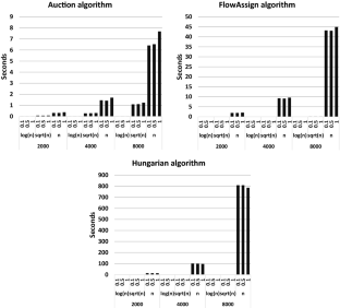
First, we give a detailed review of two algorithms that solve the minimization case of the assignment problem, the Bertsekas auction algorithm and the Goldberg & Kennedy algorithm. It was previously alluded that both algorithms are equivalent. We give a detailed proof that these algorithms are equivalent. Also, we perform experimental results comparing the performance of three algorithms for the assignment problem: the \(\epsilon \) - scaling auction algorithm , the Hungarian algorithm and the FlowAssign algorithm . The experiment shows that the auction algorithm still performs and scales better in practice than the other algorithms which are harder to implement and have better theoretical time complexity.

This is a preview of subscription content, log in via an institution to check access.

Access this article

Price includes VAT (Russian Federation)

Instant access to the full article PDF.

Rent this article via DeepDyve

Institutional subscriptions

Similar content being viewed by others

Some results on an assignment problem variant

Pritibhushan Sinha

Integer Programming

A Full Description of Polytopes Related to the Index of the Lowest Nonzero Row of an Assignment Matrix

Bertsekas, D.P.: The auction algorithm: a distributed relaxation method for the assignment problem. Annal Op. Res. 14 , 105–123 (1988)

Article   MathSciNet   Google Scholar  

Bertsekas, D.P., Castañon, D.A.: Parallel synchronous and asynchronous implementations of the auction algorithm. Parallel Comput. 17 , 707–732 (1991)

Article   Google Scholar  

Bertsekas, D.P.: Linear network optimization: algorithms and codes. MIT Press, Cambridge, MA (1991)

MATH   Google Scholar  

Bertsekas, D.P.: The auction algorithm for shortest paths. SIAM J. Optim. 1 , 425–477 (1991)

Bertsekas, D.P.: Auction algorithms for network flow problems: a tutorial introduction. Comput. Optim. Appl. 1 , 7–66 (1992)

Bertsekas, D.P., Castañon, D.A., Tsaknakis, H.: Reverse auction and the solution of inequality constrained assignment problems. SIAM J. Optim. 3 , 268–299 (1993)

Bertsekas, D.P., Eckstein, J.: Dual coordinate step methods for linear network flow problems. Math. Progr., Ser. B 42 , 203–243 (1988)

Bertsimas, D., Tsitsiklis, J.N.: Introduction to linear optimization. Athena Scientific, Belmont, MA (1997)

Google Scholar  

Burkard, R., Dell’Amico, M., Martello, S.: Assignment Problems. Revised reprint. SIAM, Philadelphia, PA (2011)

Gabow, H.N., Tarjan, R.E.: Faster scaling algorithms for network problems. SIAM J. Comput. 18 (5), 1013–1036 (1989)

Goldberg, A.V., Tarjan, R.E.: A new approach to the maximum flow problem. J. Assoc. Comput. Mach. 35 , 921–940 (1988)

Goldberg, A.V., Tarjan, R.E.: Finding minimum-cost circulations by successive approximation. Math. Op. Res. 15 , 430–466 (1990)

Goldberg, A.V., Kennedy, R.: An efficient cost scaling algorithm for the assignment problem. Math. Programm. 71 , 153–177 (1995)

MathSciNet   MATH   Google Scholar  

Goldberg, A.V., Kennedy, R.: Global price updates help. SIAM J. Discr. Math. 10 (4), 551–572 (1997)

Kuhn, H.W.: The Hungarian method for the assignment problem. Naval Res. Logist. Quart. 2 , 83–97 (1955)

Kuhn, H.W.: Variants of the Hungarian method for the assignment problem. Naval Res. Logist. Quart. 2 , 253–258 (1956)

Lawler, E.L.: Combinatorial optimization: networks and matroids, Holt. Rinehart & Winston, New York (1976)

Orlin, J.B., Ahuja, R.K.: New scaling algorithms for the assignment ad minimum mean cycle problems. Math. Programm. 54 , 41–56 (1992)

Ramshaw, L., Tarjan, R.E., Weight-Scaling Algorithm, A., for Min-Cost Imperfect Matchings in Bipartite Graphs, : IEEE 53rd Annual Symposium on Foundations of Computer Science. New Brunswick, NJ 2012 , 581–590 (2012)

Zaki, H.: A comparison of two algorithms for the assignment problem. Comput. Optim. Appl. 4 , 23–45 (1995)

Download references

Acknowledgements

This research was partially supported by SNI and CONACyT.

Author information

Authors and affiliations.

Banco de México, Mexico City, Mexico

Carlos A. Alfaro & Marcos C. Vargas

Mountain View, CA, 94043, USA

Sergio L. Perez

Departamento de Matemáticas, CINVESTAV del IPN, Apartado postal 14-740, 07000, Mexico City, Mexico

Carlos E. Valencia

You can also search for this author in PubMed   Google Scholar

Corresponding author

Correspondence to Carlos A. Alfaro .

Ethics declarations

Conflict of interest.

There is no conflict of interest.

Additional information

Publisher's note.

Springer Nature remains neutral with regard to jurisdictional claims in published maps and institutional affiliations.

The authors were partially supported by SNI and CONACyT.

Rights and permissions

Reprints and permissions

About this article

Alfaro, C.A., Perez, S.L., Valencia, C.E. et al. The assignment problem revisited. Optim Lett 16 , 1531–1548 (2022). https://doi.org/10.1007/s11590-021-01791-4

Download citation

Received : 26 March 2020

Accepted : 03 August 2021

Published : 16 August 2021

Issue Date : June 2022

DOI : https://doi.org/10.1007/s11590-021-01791-4

Share this article

Anyone you share the following link with will be able to read this content:

Sorry, a shareable link is not currently available for this article.

Provided by the Springer Nature SharedIt content-sharing initiative

• Assignment problem
• Bertsekas auction algorithm
• Combinatorial optimization and matching
• Find a journal
• Publish with us
• Track your research

Assignment Problem: Maximization

There are problems where certain facilities have to be assigned to a number of jobs, so as to maximize the overall performance of the assignment.

The Hungarian Method can also solve such assignment problems , as it is easy to obtain an equivalent minimization problem by converting every number in the matrix to an opportunity loss.

The conversion is accomplished by subtracting all the elements of the given matrix from the highest element. It turns out that minimizing opportunity loss produces the same assignment solution as the original maximization problem.

• Unbalanced Assignment Problem
• Multiple Optimal Solutions

Example: Maximization In An Assignment Problem

At the head office of www.universalteacherpublications.com there are five registration counters. Five persons are available for service.

How should the counters be assigned to persons so as to maximize the profit ?

Here, the highest value is 62. So we subtract each value from 62. The conversion is shown in the following table.

On small screens, scroll horizontally to view full calculation

Now the above problem can be easily solved by Hungarian method . After applying steps 1 to 3 of the Hungarian method, we get the following matrix.

Draw the minimum number of vertical and horizontal lines necessary to cover all the zeros in the reduced matrix.

Select the smallest element from all the uncovered elements, i.e., 4. Subtract this element from all the uncovered elements and add it to the elements, which lie at the intersection of two lines. Thus, we obtain another reduced matrix for fresh assignment. Repeating step 3, we obtain a solution which is shown in the following table.

Final Table: Maximization Problem

Use Horizontal Scrollbar to View Full Table Calculation

The total cost of assignment = 1C + 2E + 3A + 4D + 5B

Substituting values from original table: 40 + 36 + 40 + 36 + 62 = 214.

Share This Article

Operations Research Simplified Back Next

Goal programming Linear programming Simplex Method Transportation Problem

How to Solve the Assignment Problem: A Complete Guide

Table of Contents

Assignment problem is a special type of linear programming problem that deals with assigning a number of resources to an equal number of tasks in the most efficient way. The goal is to minimize the total cost of assignments while ensuring that each task is assigned to only one resource and each resource is assigned to only one task. In this blog, we will discuss the solution of the assignment problem using the Hungarian method, which is a popular algorithm for solving the problem.

Understanding the Assignment Problem

Before we dive into the solution, it is important to understand the problem itself. In the assignment problem, we have a matrix of costs, where each row represents a resource and each column represents a task. The objective is to assign each resource to a task in such a way that the total cost of assignments is minimized. However, there are certain constraints that need to be satisfied – each resource can be assigned to only one task and each task can be assigned to only one resource.

Solving the Assignment Problem

There are various methods for solving the assignment problem, including the Hungarian method, the brute force method, and the auction algorithm. Here, we will focus on the steps involved in solving the assignment problem using the Hungarian method, which is the most commonly used and efficient method.

Step 1: Set up the cost matrix

The first step in solving the assignment problem is to set up the cost matrix, which represents the cost of assigning a task to an agent. The matrix should be square and have the same number of rows and columns as the number of tasks and agents, respectively.

Step 2: Subtract the smallest element from each row and column

To simplify the calculations, we need to reduce the size of the cost matrix by subtracting the smallest element from each row and column. This step is called matrix reduction.

Step 3: Cover all zeros with the minimum number of lines

The next step is to cover all zeros in the matrix with the minimum number of horizontal and vertical lines. This step is called matrix covering.

Step 4: Test for optimality and adjust the matrix

To test for optimality, we need to calculate the minimum number of lines required to cover all zeros in the matrix. If the number of lines equals the number of rows or columns, the solution is optimal. If not, we need to adjust the matrix and repeat steps 3 and 4 until we get an optimal solution.

Step 5: Assign the tasks to the agents

The final step is to assign the tasks to the agents based on the optimal solution obtained in step 4. This will give us the most cost-effective or profit-maximizing assignment.

Solution of the Assignment Problem using the Hungarian Method

The Hungarian method is an algorithm that uses a step-by-step approach to find the optimal assignment. The algorithm consists of the following steps:

• Subtract the smallest entry in each row from all the entries of the row.
• Subtract the smallest entry in each column from all the entries of the column.
• Draw the minimum number of lines to cover all zeros in the matrix. If the number of lines drawn is equal to the number of rows, we have an optimal solution. If not, go to step 4.
• Determine the smallest entry not covered by any line. Subtract it from all uncovered entries and add it to all entries covered by two lines. Go to step 3.

The above steps are repeated until an optimal solution is obtained. The optimal solution will have all zeros covered by the minimum number of lines. The assignments can be made by selecting the rows and columns with a single zero in the final matrix.

Applications of the Assignment Problem

The assignment problem has various applications in different fields, including computer science, economics, logistics, and management. In this section, we will provide some examples of how the assignment problem is used in real-life situations.

Applications in Computer Science

The assignment problem can be used in computer science to allocate resources to different tasks, such as allocating memory to processes or assigning threads to processors.

Applications in Economics

The assignment problem can be used in economics to allocate resources to different agents, such as allocating workers to jobs or assigning projects to contractors.

Applications in Logistics

The assignment problem can be used in logistics to allocate resources to different activities, such as allocating vehicles to routes or assigning warehouses to customers.

Applications in Management

The assignment problem can be used in management to allocate resources to different projects, such as allocating employees to tasks or assigning budgets to departments.

Let’s consider the following scenario: a manager needs to assign three employees to three different tasks. Each employee has different skills, and each task requires specific skills. The manager wants to minimize the total time it takes to complete all the tasks. The skills and the time required for each task are given in the table below:

The assignment problem is to determine which employee should be assigned to which task to minimize the total time required. To solve this problem, we can use the Hungarian method, which we discussed in the previous blog.

Using the Hungarian method, we first subtract the smallest entry in each row from all the entries of the row:

Next, we subtract the smallest entry in each column from all the entries of the column:

We draw the minimum number of lines to cover all the zeros in the matrix, which in this case is three:

Since the number of lines is equal to the number of rows, we have an optimal solution. The assignments can be made by selecting the rows and columns with a single zero in the final matrix. In this case, the optimal assignments are:

• Emp 1 to Task 3
• Emp 2 to Task 2
• Emp 3 to Task 1

This assignment results in a total time of 9 units.

I hope this example helps you better understand the assignment problem and how to solve it using the Hungarian method.

Solving the assignment problem may seem daunting, but with the right approach, it can be a straightforward process. By following the steps outlined in this guide, you can confidently tackle any assignment problem that comes your way.

How useful was this post?

Click on a star to rate it!

Average rating 0 / 5. Vote count: 0

No votes so far! Be the first to rate this post.

We are sorry that this post was not useful for you! 😔

Let us improve this post!

Tell us how we can improve this post?

Operations Research

1 Operations Research-An Overview

• History of O.R.
• Approach, Techniques and Tools
• Phases and Processes of O.R. Study
• Typical Applications of O.R
• Limitations of Operations Research
• Models in Operations Research
• O.R. in real world

2 Linear Programming: Formulation and Graphical Method

• General formulation of Linear Programming Problem
• Optimisation Models
• Basics of Graphic Method
• Important steps to draw graph
• Multiple, Unbounded Solution and Infeasible Problems
• Solving Linear Programming Graphically Using Computer
• Application of Linear Programming in Business and Industry

3 Linear Programming-Simplex Method

• Principle of Simplex Method
• Computational aspect of Simplex Method
• Simplex Method with several Decision Variables
• Two Phase and M-method
• Multiple Solution, Unbounded Solution and Infeasible Problem
• Sensitivity Analysis
• Dual Linear Programming Problem

4 Transportation Problem

• Basic Feasible Solution of a Transportation Problem
• Modified Distribution Method
• Stepping Stone Method
• Unbalanced Transportation Problem
• Degenerate Transportation Problem
• Transhipment Problem
• Maximisation in a Transportation Problem

5 Assignment Problem

• Solution of the Assignment Problem
• Unbalanced Assignment Problem
• Problem with some Infeasible Assignments
• Maximisation in an Assignment Problem
• Crew Assignment Problem

6 Application of Excel Solver to Solve LPP

• Building Excel model for solving LP: An Illustrative Example

7 Goal Programming

• Concepts of goal programming
• Goal programming model formulation
• Graphical method of goal programming
• The simplex method of goal programming
• Using Excel Solver to Solve Goal Programming Models
• Application areas of goal programming

8 Integer Programming

• Some Integer Programming Formulation Techniques
• Binary Representation of General Integer Variables
• Unimodularity
• Cutting Plane Method
• Branch and Bound Method
• Solver Solution

9 Dynamic Programming

• Dynamic Programming Methodology: An Example
• Definitions and Notations
• Dynamic Programming Applications

10 Non-Linear Programming

• Solution of a Non-linear Programming Problem
• Convex and Concave Functions
• Kuhn-Tucker Conditions for Constrained Optimisation
• Quadratic Programming
• Separable Programming
• NLP Models with Solver

11 Introduction to game theory and its Applications

• Important terms in Game Theory
• Saddle points
• Mixed strategies: Games without saddle points
• 2 x n games
• Exploiting an opponent’s mistakes

12 Monte Carlo Simulation

• Reasons for using simulation
• Monte Carlo simulation
• Limitations of simulation
• Steps in the simulation process
• Some practical applications of simulation
• Two typical examples of hand-computed simulation
• Computer simulation

13 Queueing Models

• Characteristics of a queueing model
• Notations and Symbols
• Statistical methods in queueing
• The M/M/I System
• The M/M/C System
• The M/Ek/I System
• Decision problems in queueing

• school Campus Bookshelves
• menu_book Bookshelves
• perm_media Learning Objects
• login Login
• how_to_reg Request Instructor Account
• hub Instructor Commons
• Download Page (PDF)
• Download Full Book (PDF)
• Periodic Table
• Physics Constants
• Scientific Calculator
• Reference & Cite
• Tools expand_more
• Readability

selected template will load here

This action is not available.

6.4.3.1: Minimization By The Simplex Method (Exercises)

• Last updated
• Save as PDF
• Page ID 26554

• Rupinder Sekhon and Roberta Bloom
• De Anza College

SECTION 6.4.3 PROBLEM SET: MINIMIZATION BY THE SIMPLEX METHOD

In problems 1-2, convert each minimization problem into a maximization problem, the dual, and then solve by the simplex method.

1) \[\begin{aligned} \text { Minimize } & \mathrm{z}=6 \mathrm{x}_{1}+8 \mathrm{x}_{2} \\ \text { subject to } & 2 \mathrm{x}_{1}+3 \mathrm{x}_{2} \geq 7 \\ & 4 \mathrm{x}_{1}+5 \mathrm{x}_{2} \geq 9 \\ & \mathrm{x}_{1}, \mathrm{x}_{2} \geq 0 \end{aligned} \nonumber \]

2) \[\begin{array}{ll} \text { Minimize } & \mathrm{z}=5 \mathrm{x}_{1}+6 \mathrm{x}_{2}+7 \mathrm{x}_{3} \\ \text { subject to } & 3 \mathrm{x}_{1}+2 \mathrm{x}_{2}+3 \mathrm{x}_{3} \quad \geq 10 \\ & 4 \mathrm{x}_{1}+3 \mathrm{x}_{2}+5 \mathrm{x}_{3} \geq 12 \\ &\mathrm{x}_{1}, \mathrm{x}_{2}, \mathrm{x}_{3} \geq & 0 \end{array} \nonumber \]

In problems 3-4, convert each minimization problem into a maximization problem, the dual, and then solve by the simplex method.

3) \[\begin{array}{lr} \text { Minimize } & \mathrm{z}=4 \mathrm{x}_1+3 \mathrm{x}_2 \\ \text { subject to } & \mathrm{x}_{1}+\mathrm{x}_{2} \geq 10 \\ & 3 \mathrm{x}_{1}+2 \mathrm{x}_{2} \geq 24 \\ & \mathrm{x}_{1}, \mathrm{x}_{2} \geq 0 \end{array} \nonumber \]

4) A diet is to contain at least 8 units of vitamins, 9 units of minerals, and 10 calories. Three foods, Food A, Food B, and Food C are to be purchased. Each unit of Food A provides 1 unit of vitamins, 1 unit of minerals, and 2 calories. Each unit of Food B provides 2 units of vitamins, 1 unit of minerals, and 1 calorie. Each unit of Food C provides 2 units of vitamins, 1 unit of minerals, and 2 calories. If Food A costs $3 per unit, Food B costs $2 per unit and Food C costs $3 per unit, how many units of each food should be purchased to keep costs at a minimum?

Procedure, Example Solved Problem | Operations Research - Solution of assignment problems (Hungarian Method) | 12th Business Maths and Statistics : Chapter 10 : Operations Research

Chapter: 12th business maths and statistics : chapter 10 : operations research.

Solution of assignment problems (Hungarian Method)

First check whether the number of rows is equal to the numbers of columns, if it is so, the assignment problem is said to be balanced.

Step :1 Choose the least element in each row and subtract it from all the elements of that row.

Step :2 Choose the least element in each column and subtract it from all the elements of that column. Step 2 has to be performed from the table obtained in step 1.

Step:3 Check whether there is atleast one zero in each row and each column and make an assignment as follows.

Step :4 If each row and each column contains exactly one assignment, then the solution is optimal.

Example 10.7

Solve the following assignment problem. Cell values represent cost of assigning job A, B, C and D to the machines I, II, III and IV.

Here the number of rows and columns are equal.

∴ The given assignment problem is balanced. Now let us find the solution.

Step 1: Select a smallest element in each row and subtract this from all the elements in its row.

Look for atleast one zero in each row and each column.Otherwise go to step 2.

Step 2: Select the smallest element in each column and subtract this from all the elements in its column.

Since each row and column contains atleast one zero, assignments can be made.

Step 3 (Assignment):

Thus all the four assignments have been made. The optimal assignment schedule and total cost is

The optimal assignment (minimum) cost

Example 10.8

Consider the problem of assigning five jobs to five persons. The assignment costs are given as follows. Determine the optimum assignment schedule.

∴ The given assignment problem is balanced.

Now let us find the solution.

The cost matrix of the given assignment problem is

Column 3 contains no zero. Go to Step 2.

Thus all the five assignments have been made. The Optimal assignment schedule and total cost is

The optimal assignment (minimum) cost = ` 9

Example 10.9

Solve the following assignment problem.

Since the number of columns is less than the number of rows, given assignment problem is unbalanced one. To balance it , introduce a dummy column with all the entries zero. The revised assignment problem is

Here only 3 tasks can be assigned to 3 men.

Step 1: is not necessary, since each row contains zero entry. Go to Step 2.

Step 3 (Assignment) :

Since each row and each columncontains exactly one assignment,all the three men have been assigned a task. But task S is not assigned to any Man. The optimal assignment schedule and total cost is

The optimal assignment (minimum) cost = ₹ 35

Related Topics

Privacy Policy , Terms and Conditions , DMCA Policy and Compliant

Copyright © 2018-2024 BrainKart.com; All Rights Reserved. Developed by Therithal info, Chennai.

• school Campus Bookshelves
• menu_book Bookshelves
• perm_media Learning Objects
• login Login
• how_to_reg Request Instructor Account
• hub Instructor Commons
• Download Page (PDF)
• Download Full Book (PDF)
• Periodic Table
• Physics Constants
• Scientific Calculator
• Reference & Cite
• Tools expand_more
• Readability

selected template will load here

This action is not available.

4.7: Optimization Problems

• Last updated
• Save as PDF
• Page ID 4467

Learning Objectives

• Set up and solve optimization problems in several applied fields.

One common application of calculus is calculating the minimum or maximum value of a function. For example, companies often want to minimize production costs or maximize revenue. In manufacturing, it is often desirable to minimize the amount of material used to package a product with a certain volume. In this section, we show how to set up these types of minimization and maximization problems and solve them by using the tools developed in this chapter.

Solving Optimization Problems over a Closed, Bounded Interval

The basic idea of the optimization problems that follow is the same. We have a particular quantity that we are interested in maximizing or minimizing. However, we also have some auxiliary condition that needs to be satisfied. For example, in Example \(\PageIndex{1}\), we are interested in maximizing the area of a rectangular garden. Certainly, if we keep making the side lengths of the garden larger, the area will continue to become larger. However, what if we have some restriction on how much fencing we can use for the perimeter? In this case, we cannot make the garden as large as we like. Let’s look at how we can maximize the area of a rectangle subject to some constraint on the perimeter.

Example \(\PageIndex{1}\): Maximizing the Area of a Garden

A rectangular garden is to be constructed using a rock wall as one side of the garden and wire fencing for the other three sides (Figure \(\PageIndex{1}\)). Given \(100\,\text{ft}\) of wire fencing, determine the dimensions that would create a garden of maximum area. What is the maximum area?

Let \(x\) denote the length of the side of the garden perpendicular to the rock wall and \(y\) denote the length of the side parallel to the rock wall. Then the area of the garden is

\(A=x⋅y.\)

We want to find the maximum possible area subject to the constraint that the total fencing is \(100\,\text{ft}\). From Figure \(\PageIndex{1}\), the total amount of fencing used will be \(2x+y.\) Therefore, the constraint equation is

\(2x+y=100.\)

Solving this equation for \(y\), we have \(y=100−2x.\) Thus, we can write the area as

\(A(x)=x⋅(100−2x)=100x−2x^2.\)

Before trying to maximize the area function \(A(x)=100x−2x^2,\) we need to determine the domain under consideration. To construct a rectangular garden, we certainly need the lengths of both sides to be positive. Therefore, we need \(x>0\) and \(y>0\). Since \(y=100−2x\), if \(y>0\), then \(x<50\). Therefore, we are trying to determine the maximum value of \(A(x)\) for \(x\) over the open interval \((0,50)\). We do not know that a function necessarily has a maximum value over an open interval. However, we do know that a continuous function has an absolute maximum (and absolute minimum) over a closed interval. Therefore, let’s consider the function \(A(x)=100x−2x^2\) over the closed interval \([0,50]\). If the maximum value occurs at an interior point, then we have found the value \(x\) in the open interval \((0,50)\) that maximizes the area of the garden.

Therefore, we consider the following problem:

Maximize \(A(x)=100x−2x^2\) over the interval \([0,50].\)

As mentioned earlier, since \(A\) is a continuous function on a closed, bounded interval, by the extreme value theorem, it has a maximum and a minimum. These extreme values occur either at endpoints or critical points. At the endpoints, \(A(x)=0\). Since the area is positive for all \(x\) in the open interval \((0,50)\), the maximum must occur at a critical point. Differentiating the function \(A(x)\), we obtain

\(A′(x)=100−4x.\)

Therefore, the only critical point is \(x=25\) (Figure \(\PageIndex{2}\)). We conclude that the maximum area must occur when \(x=25\).

Then we have \(y=100−2x=100−2(25)=50.\) To maximize the area of the garden, let \(x=25\,\text{ft}\) and \(y=50\,\text{ft}\). The area of this garden is \(1250\, \text{ft}^2\).

Exercise \(\PageIndex{1}\)

Determine the maximum area if we want to make the same rectangular garden as in Figure \(\PageIndex{2}\), but we have \(200\,\text{ft}\) of fencing.

We need to maximize the function \(A(x)=200x−2x^2\) over the interval \([0,100].\)

The maximum area is \(5000\, \text{ft}^2\).

Now let’s look at a general strategy for solving optimization problems similar to Example \(\PageIndex{1}\).

Problem-Solving Strategy: Solving Optimization Problems

• Introduce all variables. If applicable, draw a figure and label all variables.
• Determine which quantity is to be maximized or minimized, and for what range of values of the other variables (if this can be determined at this time).
• Write a formula for the quantity to be maximized or minimized in terms of the variables. This formula may involve more than one variable.
• Write any equations relating the independent variables in the formula from step \(3\). Use these equations to write the quantity to be maximized or minimized as a function of one variable.
• Identify the domain of consideration for the function in step \(4\) based on the physical problem to be solved.
• Locate the maximum or minimum value of the function from step \(4.\) This step typically involves looking for critical points and evaluating a function at endpoints.

Now let’s apply this strategy to maximize the volume of an open-top box given a constraint on the amount of material to be used.

Example \(\PageIndex{2}\): Maximizing the Volume of a Box

An open-top box is to be made from a \(24\,\text{in.}\) by \(36\,\text{in.}\) piece of cardboard by removing a square from each corner of the box and folding up the flaps on each side. What size square should be cut out of each corner to get a box with the maximum volume?

Step 1: Let \(x\) be the side length of the square to be removed from each corner (Figure \(\PageIndex{3}\)). Then, the remaining four flaps can be folded up to form an open-top box. Let \(V\) be the volume of the resulting box.

Step 2: We are trying to maximize the volume of a box. Therefore, the problem is to maximize \(V\).

Step 3: As mentioned in step 2, are trying to maximize the volume of a box. The volume of a box is

\[V=L⋅W⋅H \nonumber, \nonumber \]

where \(L,\,W,\)and \(H\) are the length, width, and height, respectively.

Step 4: From Figure \(\PageIndex{3}\), we see that the height of the box is \(x\) inches, the length is \(36−2x\) inches, and the width is \(24−2x\) inches. Therefore, the volume of the box is

\[ \begin{align*} V(x) &=(36−2x)(24−2x)x \\[4pt] &=4x^3−120x^2+864x \end{align*}. \nonumber \]

Step 5: To determine the domain of consideration, let’s examine Figure \(\PageIndex{3}\). Certainly, we need \(x>0.\) Furthermore, the side length of the square cannot be greater than or equal to half the length of the shorter side, \(24\,\text{in.}\); otherwise, one of the flaps would be completely cut off. Therefore, we are trying to determine whether there is a maximum volume of the box for \(x\) over the open interval \((0,12).\) Since \(V\) is a continuous function over the closed interval \([0,12]\), we know \(V\) will have an absolute maximum over the closed interval. Therefore, we consider \(V\) over the closed interval \([0,12]\) and check whether the absolute maximum occurs at an interior point.

Step 6: Since \(V(x)\) is a continuous function over the closed, bounded interval \([0,12]\), \(V\) must have an absolute maximum (and an absolute minimum). Since \(V(x)=0\) at the endpoints and \(V(x)>0\) for \(0<x<12,\) the maximum must occur at a critical point. The derivative is

\(V′(x)=12x^2−240x+864.\)

To find the critical points, we need to solve the equation

\(12x^2−240x+864=0.\)

Dividing both sides of this equation by \(12\), the problem simplifies to solving the equation

\(x^2−20x+72=0.\)

Using the quadratic formula, we find that the critical points are

\[\begin{align*} x &=\dfrac{20±\sqrt{(−20)^2−4(1)(72)}}{2} \\[4pt] &=\dfrac{20±\sqrt{112}}{2} \\[4pt] &=\dfrac{20±4\sqrt{7}}{2} \\[4pt] &=10±2\sqrt{7} \end{align*}. \nonumber \]

Since \(10+2\sqrt{7}\) is not in the domain of consideration, the only critical point we need to consider is \(10−2\sqrt{7}\). Therefore, the volume is maximized if we let \(x=10−2\sqrt{7}\,\text{in.}\) The maximum volume is

\[V(10−2\sqrt{7})=640+448\sqrt{7}≈1825\,\text{in}^3. \nonumber \]

as shown in the following graph.

Exercise \(\PageIndex{2}\)

Suppose the dimensions of the cardboard in Example \(\PageIndex{2}\) are \(20\,\text{in.}\) by \(30\,\text{in.}\) Let \(x\) be the side length of each square and write the volume of the open-top box as a function of \(x\). Determine the domain of consideration for \(x\).

The volume of the box is \(L⋅W⋅H.\)

\(V(x)=x(20−2x)(30−2x).\) The domain is \([0,10]\).

Example \(\PageIndex{3}\): Minimizing Travel Time

An island is \(2\) mi due north of its closest point along a straight shoreline. A visitor is staying at a cabin on the shore that is \(6\) mi west of that point. The visitor is planning to go from the cabin to the island. Suppose the visitor runs at a rate of \(8\) mph and swims at a rate of \(3\) mph. How far should the visitor run before swimming to minimize the time it takes to reach the island?

Step 1: Let \(x\) be the distance running and let \(y\) be the distance swimming (Figure \(\PageIndex{5}\)). Let \(T\) be the time it takes to get from the cabin to the island.

Step 2: The problem is to minimize \(T\).

Step 3: To find the time spent traveling from the cabin to the island, add the time spent running and the time spent swimming. Since Distance = Rate × Time \((D=R×T),\) the time spent running is

\(T_{running}=\dfrac{D_{running}}{R_{running}}=\dfrac{x}{8}\),

and the time spent swimming is

\(T_{swimming}=\dfrac{D_{swimming}}{R_{swimming}}=\dfrac{y}{3}\).

Therefore, the total time spent traveling is

\(T=\dfrac{x}{8}+\dfrac{y}{3}\).

Step 4: From Figure \(\PageIndex{5}\), the line segment of \(y\) miles forms the hypotenuse of a right triangle with legs of length \(2\) mi and \(6−x\) mi. Therefore, by the Pythagorean theorem, \(2^2+(6−x)^2=y^2\), and we obtain \(y=\sqrt{(6−x)^2+4}\). Thus, the total time spent traveling is given by the function

\(T(x)=\dfrac{x}{8}+\dfrac{\sqrt{(6−x)^2+4}}{3}\).

Step 5: From Figure \(\PageIndex{5}\), we see that \(0≤x≤6\). Therefore, \([0,6]\) is the domain of consideration.

Step 6: Since \(T(x)\) is a continuous function over a closed, bounded interval, it has a maximum and a minimum. Let’s begin by looking for any critical points of \(T\) over the interval \([0,6].\) The derivative is

\[\begin{align*} T′(x) &=\dfrac{1}{8}−\dfrac{1}{2}\dfrac{[(6−x)^2+4]^{−1/2}}{3}⋅2(6−x) \\[4pt] &=\dfrac{1}{8}−\dfrac{(6−x)}{3\sqrt{(6−x)^2+4}} \end{align*}\]

If \(T′(x)=0,\), then

\[\dfrac{1}{8}=\dfrac{6−x}{3\sqrt{(6−x)^2+4}} \label{ex3eq1} \]

\[3\sqrt{(6−x)^2+4}=8(6−x). \label{ex3eq2} \]

Squaring both sides of this equation, we see that if \(x\) satisfies this equation, then \(x\) must satisfy

\[9[(6−x)^2+4]=64(6−x)^2,\nonumber \]

which implies

\[55(6−x)^2=36. \nonumber \]

We conclude that if \(x\) is a critical point, then \(x\) satisfies

\[(x−6)^2=\dfrac{36}{55}. \nonumber \]

[Note that since we are squaring, \( (x-6)^2 = (6-x)^2.\)]

Therefore, the possibilities for critical points are

\[x=6±\dfrac{6}{\sqrt{55}}.\nonumber \]

Since \(x=6+6/\sqrt{55}\) is not in the domain, it is not a possibility for a critical point. On the other hand, \(x=6−6/\sqrt{55}\) is in the domain. Since we squared both sides of Equation \ref{ex3eq2} to arrive at the possible critical points, it remains to verify that \(x=6−6/\sqrt{55}\) satisfies Equation \ref{ex3eq1}. Since \(x=6−6/\sqrt{55}\) does satisfy that equation, we conclude that \(x=6−6/\sqrt{55}\) is a critical point, and it is the only one. To justify that the time is minimized for this value of \(x\), we just need to check the values of \(T(x)\) at the endpoints \(x=0\) and \(x=6\), and compare them with the value of \(T(x)\) at the critical point \(x=6−6/\sqrt{55}\). We find that \(T(0)≈2.108\,\text{h}\) and \(T(6)≈1.417\,\text{h}\), whereas

\[T(6−6/\sqrt{55})≈1.368\,\text{h}. \nonumber \]

Therefore, we conclude that \(T\) has a local minimum at \(x≈5.19\) mi.

Exercise \(\PageIndex{3}\)

Suppose the island is \(1\) mi from shore, and the distance from the cabin to the point on the shore closest to the island is \(15\) mi. Suppose a visitor swims at the rate of \(2.5\) mph and runs at a rate of \(6\) mph. Let \(x\) denote the distance the visitor will run before swimming, and find a function for the time it takes the visitor to get from the cabin to the island.

The time \(T=T_{running}+T_{swimming}.\)

\(T(x)=\dfrac{x}{6}+\dfrac{\sqrt{(15−x)^2+1}}{2.5} \)

In business, companies are interested in maximizing revenue. In the following example, we consider a scenario in which a company has collected data on how many cars it is able to lease, depending on the price it charges its customers to rent a car. Let’s use these data to determine the price the company should charge to maximize the amount of money it brings in.

Example \(\PageIndex{4}\): Maximizing Revenue

Owners of a car rental company have determined that if they charge customers \(p\) dollars per day to rent a car, where \(50≤p≤200\), the number of cars \(n\) they rent per day can be modeled by the linear function \(n(p)=1000−5p\). If they charge \($50\) per day or less, they will rent all their cars. If they charge \($200\) per day or more, they will not rent any cars. Assuming the owners plan to charge customers between \($50\) per day and \($200\) per day to rent a car, how much should they charge to maximize their revenue?

Step 1: Let \(p\) be the price charged per car per day and let \(n\) be the number of cars rented per day. Let \(R\) be the revenue per day.

Step 2: The problem is to maximize \(R.\)

Step 3: The revenue (per day) is equal to the number of cars rented per day times the price charged per car per day—that is, \(R=n×p.\)

Step 4: Since the number of cars rented per day is modeled by the linear function \(n(p)=1000−5p,\) the revenue \(R\) can be represented by the function

\[ \begin{align*} R(p) &=n×p \\[4pt] &=(1000−5p)p \\[4pt] &=−5p^2+1000p.\end{align*}\]

Step 5: Since the owners plan to charge between \($50\) per car per day and \($200\) per car per day, the problem is to find the maximum revenue \(R(p)\) for \(p\) in the closed interval \([50,200]\).

Step 6: Since \(R\) is a continuous function over the closed, bounded interval \([50,200]\), it has an absolute maximum (and an absolute minimum) in that interval. To find the maximum value, look for critical points. The derivative is \(R′(p)=−10p+1000.\) Therefore, the critical point is \(p=100\). When \(p=100, R(100)=$50,000.\) When \(p=50, R(p)=$37,500\). When \(p=200, R(p)=$0\).

Therefore, the absolute maximum occurs at \(p=$100\). The car rental company should charge \($100\) per day per car to maximize revenue as shown in the following figure.

Exercise \(\PageIndex{4}\)

A car rental company charges its customers \(p\) dollars per day, where \(60≤p≤150\). It has found that the number of cars rented per day can be modeled by the linear function \(n(p)=750−5p.\) How much should the company charge each customer to maximize revenue?

\(R(p)=n×p,\) where \(n\) is the number of cars rented and \(p\) is the price charged per car.

The company should charge \($75\) per car per day.

Example \(\PageIndex{5}\): Maximizing the Area of an Inscribed Rectangle

A rectangle is to be inscribed in the ellipse

\[\dfrac{x^2}{4}+y^2=1. \nonumber \]

What should the dimensions of the rectangle be to maximize its area? What is the maximum area?

Step 1: For a rectangle to be inscribed in the ellipse, the sides of the rectangle must be parallel to the axes. Let \(L\) be the length of the rectangle and \(W\) be its width. Let \(A\) be the area of the rectangle.

Step 2: The problem is to maximize \(A\).

Step 3: The area of the rectangle is \(A=LW.\)

Step 4: Let \((x,y)\) be the corner of the rectangle that lies in the first quadrant, as shown in Figure \(\PageIndex{7}\). We can write length \(L=2x\) and width \(W=2y\). Since \(\dfrac{x^2}{4}+y^2=1\) and \(y>0\), we have \(y=\sqrt{1-\dfrac{x^2}{4}}\). Therefore, the area is

\(A=LW=(2x)(2y)=4x\sqrt{1-\dfrac{x^2}{4}}=2x\sqrt{4−x^2}\)

Step 5: From Figure \(\PageIndex{7}\), we see that to inscribe a rectangle in the ellipse, the \(x\)-coordinate of the corner in the first quadrant must satisfy \(0<x<2\). Therefore, the problem reduces to looking for the maximum value of \(A(x)\) over the open interval \((0,2)\). Since \(A(x)\) will have an absolute maximum (and absolute minimum) over the closed interval \([0,2]\), we consider \(A(x)=2x\sqrt{4−x^2}\) over the interval \([0,2]\). If the absolute maximum occurs at an interior point, then we have found an absolute maximum in the open interval.

Step 6: As mentioned earlier, \(A(x)\) is a continuous function over the closed, bounded interval \([0,2]\). Therefore, it has an absolute maximum (and absolute minimum). At the endpoints \(x=0\) and \(x=2\), \(A(x)=0.\) For \(0<x<2\), \(A(x)>0\).

Therefore, the maximum must occur at a critical point. Taking the derivative of \(A(x)\), we obtain

\[ \begin{align*} A'(x) &=2\sqrt{4−x^2}+2x⋅\dfrac{1}{2\sqrt{4−x^2}}(−2x) \\[4pt] &=2\sqrt{4−x^2}−\dfrac{2x^2}{\sqrt{4−x^2}} \\[4pt] &=\dfrac{8−4x^2}{\sqrt{4−x^2}} . \end{align*}\]

To find critical points, we need to find where \(A'(x)=0.\) We can see that if \(x\) is a solution of

\[\dfrac{8−4x^2}{\sqrt{4−x^2}}=0, \label{ex5eq1} \]

then \(x\) must satisfy

\[8−4x^2=0. \nonumber \]

Therefore, \(x^2=2.\) Thus, \(x=±\sqrt{2}\) are the possible solutions of Equation \ref{ex5eq1}. Since we are considering \(x\) over the interval \([0,2]\), \(x=\sqrt{2}\) is a possibility for a critical point, but \(x=−\sqrt{2}\) is not. Therefore, we check whether \(\sqrt{2}\) is a solution of Equation \ref{ex5eq1}. Since \(x=\sqrt{2}\) is a solution of Equation \ref{ex5eq1}, we conclude that \(\sqrt{2}\) is the only critical point of \(A(x)\) in the interval \([0,2]\).

Therefore, \(A(x)\) must have an absolute maximum at the critical point \(x=\sqrt{2}\). To determine the dimensions of the rectangle, we need to find the length \(L\) and the width \(W\). If \(x=\sqrt{2}\) then

\[y=\sqrt{1−\dfrac{(\sqrt{2})^2}{4}}=\sqrt{1−\dfrac{1}{2}}=\dfrac{1}{\sqrt{2}}.\nonumber \]

Therefore, the dimensions of the rectangle are \(L=2x=2\sqrt{2}\) and \(W=2y=\dfrac{2}{\sqrt{2}}=\sqrt{2}\). The area of this rectangle is \( A=LW=(2\sqrt{2})(\sqrt{2})=4.\)

Exercise \(\PageIndex{5}\)

Modify the area function \(A\) if the rectangle is to be inscribed in the unit circle \(x^2+y^2=1\). What is the domain of consideration?

If \((x,y)\) is the vertex of the square that lies in the first quadrant, then the area of the square is \(A=(2x)(2y)=4xy.\)

\(A(x)=4x\sqrt{1−x^2}.\) The domain of consideration is \([0,1]\).

Solving Optimization Problems when the Interval Is Not Closed or Is Unbounded

In the previous examples, we considered functions on closed, bounded domains. Consequently, by the extreme value theorem, we were guaranteed that the functions had absolute extrema. Let’s now consider functions for which the domain is neither closed nor bounded.

Many functions still have at least one absolute extrema, even if the domain is not closed or the domain is unbounded. For example, the function \(f(x)=x^2+4\) over \((−∞,∞)\) has an absolute minimum of \(4\) at \(x=0\). Therefore, we can still consider functions over unbounded domains or open intervals and determine whether they have any absolute extrema. In the next example, we try to minimize a function over an unbounded domain. We will see that, although the domain of consideration is \((0,∞),\) the function has an absolute minimum.

In the following example, we look at constructing a box of least surface area with a prescribed volume. It is not difficult to show that for a closed-top box, by symmetry, among all boxes with a specified volume, a cube will have the smallest surface area. Consequently, we consider the modified problem of determining which open-topped box with a specified volume has the smallest surface area.

Example \(\PageIndex{6}\): Minimizing Surface Area

A rectangular box with a square base, an open top, and a volume of \(216 \,\text{in}^3\) is to be constructed. What should the dimensions of the box be to minimize the surface area of the box? What is the minimum surface area?

Step 1: Draw a rectangular box and introduce the variable \(x\) to represent the length of each side of the square base; let \(y\) represent the height of the box. Let \(S\) denote the surface area of the open-top box.

Step 2: We need to minimize the surface area. Therefore, we need to minimize \(S\).

Step 3: Since the box has an open top, we need only determine the area of the four vertical sides and the base. The area of each of the four vertical sides is \(x⋅y.\) The area of the base is \(x^2\). Therefore, the surface area of the box is

\(S=4xy+x^2\).

Step 4: Since the volume of this box is \(x^2y\) and the volume is given as \(216\,\text{in}^3\), the constraint equation is

\(x^2y=216\).

Solving the constraint equation for \(y\), we have \(y=\dfrac{216}{x^2}\). Therefore, we can write the surface area as a function of \(x\) only:

\[S(x)=4x\left(\dfrac{216}{x^2}\right)+x^2.\nonumber \]

Therefore, \(S(x)=\dfrac{864}{x}+x^2\).

Step 5: Since we are requiring that \(x^2y=216\), we cannot have \(x=0\). Therefore, we need \(x>0\). On the other hand, \(x\) is allowed to have any positive value. Note that as \(x\) becomes large, the height of the box \(y\) becomes correspondingly small so that \(x^2y=216\). Similarly, as \(x\) becomes small, the height of the box becomes correspondingly large. We conclude that the domain is the open, unbounded interval \((0,∞)\). Note that, unlike the previous examples, we cannot reduce our problem to looking for an absolute maximum or absolute minimum over a closed, bounded interval. However, in the next step, we discover why this function must have an absolute minimum over the interval \((0,∞).\)

Step 6: Note that as \(x→0^+,\, S(x)→∞.\) Also, as \(x→∞, \,S(x)→∞\). Since \(S\) is a continuous function that approaches infinity at the ends, it must have an absolute minimum at some \(x∈(0,∞)\). This minimum must occur at a critical point of \(S\). The derivative is

\[S′(x)=−\dfrac{864}{x^2}+2x.\nonumber \]

Therefore, \(S′(x)=0\) when \(2x=\dfrac{864}{x^2}\). Solving this equation for \(x\), we obtain \(x^3=432\), so \(x=\sqrt[3]{432}=6\sqrt[3]{2}.\) Since this is the only critical point of \(S\), the absolute minimum must occur at \(x=6\sqrt[3]{2}\) (see Figure \(\PageIndex{9}\)).

When \(x=6\sqrt[3]{2}\), \(y=\dfrac{216}{(6\sqrt[3]{2})^2}=3\sqrt[3]{2}\,\text{in.}\) Therefore, the dimensions of the box should be \(x=6\sqrt[3]{2}\,\text{in.}\) and \(y=3\sqrt[3]{2}\,\text{in.}\) With these dimensions, the surface area is

\[S(6\sqrt[3]{2})=\dfrac{864}{6\sqrt[3]{2}}+(6\sqrt[3]{2})^2=108\sqrt[3]{4}\,\text{in}^2\nonumber \]

Exercise \(\PageIndex{6}\)

Consider the same open-top box, which is to have volume \(216\,\text{in}^3\). Suppose the cost of the material for the base is \(20¢/\text{in}^2\) and the cost of the material for the sides is \(30¢/\text{in}^2\) and we are trying to minimize the cost of this box. Write the cost as a function of the side lengths of the base. (Let \(x\) be the side length of the base and \(y\) be the height of the box.)

If the cost of one of the sides is \(30¢/\text{in}^2,\) the cost of that side is \(0.30xy\) dollars.

\(c(x)=\dfrac{259.2}{x}+0.2x^2\) dollars

Key Concepts

• To solve an optimization problem, begin by drawing a picture and introducing variables.
• Find an equation relating the variables.
• Find a function of one variable to describe the quantity that is to be minimized or maximized.
• Look for critical points to locate local extrema.

• Branch and Bound Tutorial
• Backtracking Vs Branch-N-Bound
• 0/1 Knapsack
• 8 Puzzle Problem
• Job Assignment Problem
• N-Queen Problem
• Travelling Salesman Problem
• Branch and Bound Algorithm
• Introduction to Branch and Bound - Data Structures and Algorithms Tutorial
• 0/1 Knapsack using Branch and Bound
• Implementation of 0/1 Knapsack using Branch and Bound
• 8 puzzle Problem using Branch And Bound

Job Assignment Problem using Branch And Bound

• N Queen Problem using Branch And Bound
• Traveling Salesman Problem using Branch And Bound

Let there be N workers and N jobs. Any worker can be assigned to perform any job, incurring some cost that may vary depending on the work-job assignment. It is required to perform all jobs by assigning exactly one worker to each job and exactly one job to each agent in such a way that the total cost of the assignment is minimized.

Let us explore all approaches for this problem.

Solution 1: Brute Force  

We generate n! possible job assignments and for each such assignment, we compute its total cost and return the less expensive assignment. Since the solution is a permutation of the n jobs, its complexity is O(n!).

Solution 2: Hungarian Algorithm  

The optimal assignment can be found using the Hungarian algorithm. The Hungarian algorithm has worst case run-time complexity of O(n^3).

Solution 3: DFS/BFS on state space tree  

A state space tree is a N-ary tree with property that any path from root to leaf node holds one of many solutions to given problem. We can perform depth-first search on state space tree and but successive moves can take us away from the goal rather than bringing closer. The search of state space tree follows leftmost path from the root regardless of initial state. An answer node may never be found in this approach. We can also perform a Breadth-first search on state space tree. But no matter what the initial state is, the algorithm attempts the same sequence of moves like DFS.

Solution 4: Finding Optimal Solution using Branch and Bound  

The selection rule for the next node in BFS and DFS is “blind”. i.e. the selection rule does not give any preference to a node that has a very good chance of getting the search to an answer node quickly. The search for an optimal solution can often be speeded by using an “intelligent” ranking function, also called an approximate cost function to avoid searching in sub-trees that do not contain an optimal solution. It is similar to BFS-like search but with one major optimization. Instead of following FIFO order, we choose a live node with least cost. We may not get optimal solution by following node with least promising cost, but it will provide very good chance of getting the search to an answer node quickly.

There are two approaches to calculate the cost function:  

• For each worker, we choose job with minimum cost from list of unassigned jobs (take minimum entry from each row).
• For each job, we choose a worker with lowest cost for that job from list of unassigned workers (take minimum entry from each column).

In this article, the first approach is followed.

Let’s take below example and try to calculate promising cost when Job 2 is assigned to worker A. 

Since Job 2 is assigned to worker A (marked in green), cost becomes 2 and Job 2 and worker A becomes unavailable (marked in red). 

Now we assign job 3 to worker B as it has minimum cost from list of unassigned jobs. Cost becomes 2 + 3 = 5 and Job 3 and worker B also becomes unavailable. 

Finally, job 1 gets assigned to worker C as it has minimum cost among unassigned jobs and job 4 gets assigned to worker D as it is only Job left. Total cost becomes 2 + 3 + 5 + 4 = 14. 

Below diagram shows complete search space diagram showing optimal solution path in green. 

Complete Algorithm:  

Below is the implementation of the above approach:

Time Complexity: O(M*N). This is because the algorithm uses a double for loop to iterate through the M x N matrix.  Auxiliary Space: O(M+N). This is because it uses two arrays of size M and N to track the applicants and jobs.

Please Login to comment...

Similar reads.

• Branch and Bound

Improve your Coding Skills with Practice

What kind of Experience do you want to share?