inverse problem solving year 3

Year 3 | Using the Inverse Worksheets

Year 3 addition and subtraction resources

Topic: addition and subtraction

Aligned with the maths mastery approach, these  Year 3 | Using the Inverse Worksheets   are designed to save you time whilst delivering high quality learning experiences for children.

Combine with our lesson plan, maths worksheets, activity cards and revision mat for a complete maths lesson, complete with National Curriculum links, vocabulary, TAF statements, small steps, differentiation and ready to progress criteria.

Explore the rest of our year 3 addition and subtraction resources .

You May Also Like

Eyfs maths summer week 3: addition and subtraction.

Year 4 | Summer Block 1 Decimals Assessment

Year 4 | decimals: block 1: week 2 – lesson resource pack, recently viewed, tell your friends about this resource.

Get access to this and thousands of other resources with a school membership.

Check out our other sites

Privacy overview, don't have an account, sign up now, explore our new earth day resources.

Username or Email

Remember Me

Lost Password?

• Home Learning
• Free Resources
• New Resources
• Free resources
• New resources
• Filter resources
• Childrens mental health
• Easter resources

Internet Explorer is out of date!

For greater security and performance, please consider updating to one of the following free browsers

Inverse Operations – Reasoning and Problem Solving

Inverse Operations - Reasoning and Problem Solving

This worksheet includes a range of reasoning and problem solving questions for pupils to practise the main skill of finding inverse operations.

Not a member? Sign up here.

What's included in the pack? Inverse Operations reasoning and problem solving worksheet Answer sheet

National Curriculum Objectives:

(3C3) Estimate the answer to a calculation and use inverse operations to check answers

This resource is available to download with a Premium subscription.

Our Mission

To help our customers achieve a life/work balance and understand their differing needs by providing resources of outstanding quality and choice alongside excellent customer support.​.

Yes, I want that!

Keep up to date by liking our Facebook page:

Membership login, stay in touch.

01422 419608

[email protected]

Interested in getting weekly updates from us? Then sign up to our newsletter here!

Information

• Cookie Policy
• Privacy Policy
• Terms and Conditions

Copyright: Classroom Secrets 2024

Company number: 8401067

VAT number: 248 8245 74

• Terms & Conditions

Designed by Classroom Secrets

• International
• Schools directory
• Resources Jobs Schools directory News Search

Understand x 100 and ÷ 100 as inverses - Problem-Solving investigation - Year 3

Subject: Mathematics

Age range: 7-11

Resource type: Worksheet/Activity

Last updated

15 April 2024

• Share through email
• Share through twitter
• Share through linkedin
• Share through facebook
• Share through pinterest

Year 3 Place Value and Money: Understand multiplying and dividing by 10 and 100 (3-digit numbers) as inverse operations.

This in-depth maths investigation will develop maths meta-skills, and enable children to learn to think mathematically and articulate mathematical ideas.

In-depth Investigation: Lost Logic Children use their knowledge of inverse operations to solve a logic problem.

This problem-solving investigation is part of our Year 3 Place Value and Money block. Each Hamilton maths block contains a complete set of planning and resources to teach a term’s worth of objectives for one of the National Curriculum for England’s maths areas.

Tes paid licence How can I reuse this?

Get this resource as part of a bundle and save up to 36%

A bundle is a package of resources grouped together to teach a particular topic, or a series of lessons, in one place.

Year 3 Place Value - Problem-Solving Investigations

These in-depth maths investigations are open-ended problem solving activities for Year 3 children. **In-depth Investigation 1: Three Coins** Using exactly three coins, children work out how many amounts can be made between £1 and £2. **In-depth Investigation 2: Money Bags** Children use their knowledge of counting in 10s to solve a problem involving money. **In-depth Investigation: Counter Place Value** Children place counters on a place value grid to make 3-digit numbers and then use logic to ensure they have made all the combinations. **In-depth Investigation: Lost Logic** Children use their knowledge of inverse operations to solve a logic problem. **In-depth Investigation: Guess my Number** Children use their knowledge of 3-digit numbers, rounding, and properties of numbers to work out a mystery number. These investigations will develop maths meta-skills, support open-ended questioning and logical reasoning, and enable children to learn to think mathematically and articulate mathematical ideas. These problem-solving investigations come from our [Year 3 Maths Blocks](https://www.hamilton-trust.org.uk/maths/year-3-maths/). Each Hamilton maths block contains a complete set of planning and resources to teach a term’s worth of objectives for one of the National Curriculum for England’s maths areas.

Understand x 100 and ÷ 100 as inverses (Year 3 Place Value & Money)

This bundle provides three days of teaching that cover the objectives: **Understand multiplying and dividing by 10 and 100 (3-digit numbers) as inverse operations.** *Teaching Presentation* The teaching presentation includes starter activities, whole class teaching, group activities, practice sheets and mastery questions. It can be used on a variety of interactive whiteboards. *Practice Worksheets* The procedural fluency practice worksheets are differentiated for children working towards Age Related Expectations (ARE), at ARE and at greater depth. *Problem-Solving Investigation* This in-depth maths investigation will develop maths meta-skills, and enable children to learn to think mathematically and articulate mathematical ideas. *Extra Support* The extra support activity is designed to be used by a teacher or a TA with children who need extra support. This teaching is part of Hamilton’s [Year 3 Place Value and Money](https://www.hamilton-trust.org.uk/maths/year-3-maths/place-value-and-money-2/) block. Each Hamilton maths block contains a complete set of planning and resources to teach a term’s worth of objectives for one of the National Curriculum for England’s maths areas.

Your rating is required to reflect your happiness.

It's good to leave some feedback.

Something went wrong, please try again later.

This resource hasn't been reviewed yet

To ensure quality for our reviews, only customers who have purchased this resource can review it

Report this resource to let us know if it violates our terms and conditions. Our customer service team will review your report and will be in touch.

Not quite what you were looking for? Search by keyword to find the right resource:

Thank you for visiting nature.com. You are using a browser version with limited support for CSS. To obtain the best experience, we recommend you use a more up to date browser (or turn off compatibility mode in Internet Explorer). In the meantime, to ensure continued support, we are displaying the site without styles and JavaScript.

• View all journals
• My Account Login
• Explore content
• About the journal
• Publish with us
• Sign up for alerts
• Open access
• Published: 19 April 2024

An inversion problem for optical spectrum data via physics-guided machine learning

• Hwiwoo Park 1 ,
• Jun H. Park 2 &
• Jungseek Hwang 1  

Scientific Reports volume  14 , Article number:  9042 ( 2024 ) Cite this article

52 Accesses

Metrics details

• Electronic properties and materials
• Information theory and computation
• Superconducting properties and materials

We propose the regularized recurrent inference machine (rRIM), a novel machine-learning approach to solve the challenging problem of deriving the pairing glue function from measured optical spectra. The rRIM incorporates physical principles into both training and inference and affords noise robustness, flexibility with out-of-distribution data, and reduced data requirements. It effectively obtains reliable pairing glue functions from experimental optical spectra and yields promising solutions for similar inverse problems of the Fredholm integral equation of the first kind.

Introduction

Experimental and theoretical investigations on high-temperature copper-oxide (cuprate) superconductors, since their discovery over 35 years ago 1 , 2 , have afforded extensive results 3 . Despite these efforts, the microscopic electron-electron pairing mechanism for superconductivity remains elusive. In this regard, researchers have adopted innovative experimental techniques. Particularly, optical spectroscopy has the potential to elucidate the aforementioned pairing mechanisms because it is the only spectroscopic experimental method capable of providing quantitative physical quantities. The absolute pairing glue spectrum measured via optical spectroscopy may serve as a “smoking gun” evidence to address for this problem. The measured spectrum entails information concerning the pairing glue responsible for superconductivity. Extracting this glue function from the measured optical spectra via the decoding approach, which involves an inverse problem, contributes an essential aspect to the elucidation of high-temperature superconductivity.

The decoding-related inversion problem concerning physical systems is expressed as follows:

which is referred to as the generalized Allen formula 4 , 5 , 6 , 7 . Here \(1/\tau ^{\text{op}}(\omega )\) is the optical scattering rate, \(K(\omega , \Omega )\) is the kernel, and \(I^2\chi (\omega )\) is the pairing glue function, which describes interacting electrons by exchanging the force-mediating boson. Further, \(\chi (\omega )\) is the boson spectrum and I denotes the electron-boson coupling constant. The kernel is given as

This is referred to as the Shulga kernel 5 . The goal was to infer the glue function from the optical scattering rate obtained using optical spectroscopy 7 . Equation ( 1 ) can be expressed in a more general form as follows:

which is the Fredholm integral equation of the first kind. Here, \( k(t, \tau ) \) is referred to as the kernel and determined by the underlying physics of the given problem, and \(x(\tau )\) and y ( t ) are physical quantities related to each other through the integral equation. Such inverse problems occur in many areas of physics 6 , 8 , 9 and are known to be ill-posed 10 . The ill-posed nature arises from the instability of solutions in Eq. (3), where small changes in y can lead to significant changes in x . Consequently, obtaining a solution to the inverse problem becomes challenging, particularly when observations are corrupted by noise.

Conventional approaches for solving inverse problems, expressed in the form of Eq. ( 3 ) include singular value decomposition (SVD) 11 , least squares fit 12 , 13 , maximum entropy method (MEM) 6 , 7 , and Tikhonov regularization 14 . In particular, the MEM can effectively capture the key features of x , whereas the SVD and least-squares fit approaches, respectively, yield non-physical outputs and requiring a priori assumptions on the shape or size of x . At high noise levels, the MEM struggles to determine a unique amplitude 15 or or capture the peaks of x 16 . Despite its theoretical advantages in terms of convergence properties and well-defined solutions, Tikhonov regularization poses challenges with regard to the selection of appropriate regularization parameters 17 , 18 , 19 .

In recent years, machine learning approaches have frequently been applied to inverse problems of the Fredholm integral of the first kind 16 , 20 , 21 . Early approaches primarily utilized supervised learning 9 , 16 , 21 demonstrating that machine learning results were comparable or superior to those of the conventional MEM and more robust against observation noise. Regardless of their successes, they are principally model-agnostic, resembling black box models wherein the physical model is solely used for generating training data but not leveraged during the inference procedure. Consequently, these methods lack explainability or reliability in their outputs and require substantial training data to achieve competitive results. This typically does not pose any difficulty in conventional machine learning domains, such as image classification, speech recognition, and text generation, wherein vast datasets are readily available, and explainability and reliability may be relatively less critical. In contrast, in scientific domains, a sound theoretical foundation must be provided for the output of the model, and data acquisition must be cost-effective. This is particularly crucial, because the data collection often necessitates expensive experiments or extensive simulations.

Various approaches have been explored to incorporate physics in the machine learning process. Projection is applied to the outcomes of supervised learning; this imposes physical constraints on x such as normality, positivity, and compliance with the first and second moments 20 . In a prior study 22 , the forward model (Eq. ( 1 )) is added to the loss term for the training and serves as a regularizer. By utilizing the incorporated physics, these approaches can yield comparable results with significantly smaller training datasets as compared to conventional approaches. However, in these approaches, the application of physical constraints occurs at the last stage of the learning process. Consequently, they may not be sufficiently flexible to handle situations wherein the input significantly deviates from the training data. Adaptability to unseen data is crucial because the generated training data may not encompass all possible solutions, potentially leading to a bias in the output toward the training data.

To address this issue, we adopted a recurrent inference machine (RIM) 23 . Compared to other supervised approaches, RIM exhibits exceptional capability to incorporate physical constraints throughout both the learning and inference processes through an iterative process. This implies that physical principles are not applied solely at the last stage of the learning process but are integrated throughout the learning and inference stages; thus, RIM has remarkable flexibility for solving complex inverse problems. Additionally, the RIM framework automates many hand-tuned optimization operations, streamlining the training procedure and achieving improved results 23 , 24 . The RIM framework has been applied to various types of image reconstruction ranging from tomographic projections 25 to astrophysics 26 . However, conventional RIM requires modification to achieve competitive results in case of ill-posed inverse problems such as the Fredholm integral equation of the first kind. Accordingly, we developed the regularized RIM (rRIM). Furthermore, we demonstrated that the rRIM framework is equivalent to iterative Tikhonov regularization 27 , 28 , 29 .

The proposed physics-guided approach significantly reduces the amount of training data required, typically by several orders of magnitude. To illustrate this aspect, we quantitatively compared the average test error losses of the rRIM with those of two widely used supervised learning approaches—a fully connected network (FCN) and convolutional neural network (CNN). Owing to the sound theoretical basis of the rRIM, it can adequately explain its outputs; this is a crucial feature in scientific applications and in contrast with purely data-driven black box models. We demonstrated the robustness of the rRIM in handling noisy data by comparing its performance with those of the FCN and CNN models which are well-known for their strong noise robustness compared to MEM, especially under high observational noise conditions 9 , 16 . The rRIM exhibited much better robustness than FCN and CNN for a wide range of noise levels. The rRIM exhibits superior flexibility in handling out-of-distribution (OOD) data than do the FCN and CNN approaches. The OOD data refers to data that significantly differs in characteristics, such as shape and distribution, from any of the training data. Finally, we applied the rRIM to the experimental optical spectra of optimally and overdoped Bi \(_2\) Sr \(_2\) CaCu \(_2\) \( {\text{O}}_{{8 + \delta }} \) (Bi-2122) samples. The results were shown to be comparable with those obtained using the widely employed MEM. As a result, rRIM can be a suggestive inversion method to analyze data with significant noise.

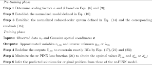
Schematic model of rRIM. Shown in blue is only used for training. Further details concerning the update network is provided in the Supplemental Material (adopted and modified from 23 ).

The generalized Allen formula, Eq. ( 1 ), can be written as

where \(F( \cdot )\) represents an integral (forward) operator. Because of the linearity of an integral operator, this equation can be discretized into the following matrix equation:

For notational simplicity, we represent the glue function and optical scattering rate as \( x \in {\mathbb {R}}^n\) and \(y \in {\mathbb {R}}^m \) , respectively. A is an \(m \times n\) matrix containing the kernel information in Eq. ( 2 ). Considering the noise in the experiment, Eq. ( 4 ) can be written as

where \(\eta \) follows a normal distribution with zero mean and \( \sigma ^2 \) variance, that is, \(\eta \sim N(0,\sigma ^2 I)\) . As the matrix \( A \in {\mathbb {R}}^{ m \times n } \) is often under-determined \( (m < n) \) and/or ill-conditioned (i.e., many of its singular values are close to 0), inferring x from y requires additional assumption on the structure of x . On this basis, the goal of the inverse problem is formulated as follows:

Notably, the solution to Eq. ( 6 ) must satisfy two constraints: it minimizes the norm \(|| \cdot ||\) and belongs to the data space \({\mathcal {X}}\) , which represents the space of proper glue functions. The norm can be chosen based on the context of the problem; in this study, we selected \(l_2\) norm.

The inverse problem expressed by Eq. ( 6 ), with the prior information on x , can be considered a maximum a posteriori (MAP) estimation 30 ,

The first term on the right-hand side represents the likelihood of the observation y given x , which is determined using the noisy forward model (Eq. ( 5 )). Further, the second term represents prior information regarding the solution space \({\mathcal {X}} \) .

The solution of the MAP estimation can be obtained using a gradient based recursive algorithm expressed as follows:

where \( l (x):= \log p(y|x) + \log p (x) \) and \( \gamma _t \) is a learning rate. Determining the appropriate learning rate is challenging. In contrast, the RIM formulates Eq. ( 7 ) as

where \(g _t \) is a deep neural network with learnable parameters \(\phi \) . More explicitly, RIM utilizes a recurrent neural network (RNN) structure as follows (Fig.  1 )

Given the observation y , the inference begins with a random initial value of \(x _0 \) . At each time step t , the gradient information \( \nabla _t := \nabla _x \log p(y|x) \vert _{x = x _t } \) is introduced into the update network \( m _{ \phi } \) along with a latent memory variable \( s _t \) . The network’s output \( g _t \) is combined with the current prediction to yield the next prediction \( x _{ t + 1 } \) . The memory variable \( s _{ t + 1 } \) , another output of \( m _{ \phi } \) , acts as a channel for the model to retain long term information, facilitating effective learning and inference during the iterative process 31 .

In the training process, the loss is calculated by comparing the training data x (shown in blue in Fig.  1 ) with the model prediction \( x _t \) at each time step. The accumulated loss is calculated formulas follows:

Here, \( w _t \) represents a positive number (in this study, we set \( w _t = 1 \) ). The parameters \(\phi \) indicate that \( x _t \) is obtained from the neural network \( m _{ \phi } \) and are updated using the backpropagation through time (BPTT) technique 32 . The solid edges in Fig.  1 illustrates the pathways for the propagation of the gradient \( \partial {\mathcal {L}}/\partial \phi \) to update \(\phi \) , whereas the dashed edges indicate the absence of gradient propagation. The trained model can perform an inference to estimate \(x _t \) given the input y without referencing the training data x .

In the conventional RIM, the gradient of the log-likelihood is given as

where \(A^{T}\) is the transpose of matrix A (see the Supplemental Material for its derivation) Owing to the inherent ill-posed nature of the aforementioned equation, it does not yield competitive results as compared to other machine learning approaches. To address this issue, we utilized the equivalence between the RIM framework and iterative Tikhonov regularization, as detailed in the Supplemental Material. Specifically, we utilized the following gradient derived from the preconditioned Landweber iteration 29 to formulate the rRIM algorithm:

Here, h is a regularization parameter. Notably, the rRIM demonstrates unique flexibility in determining the appropriate regularization parameter, a task that is typically challenging.

A few important aspects are noteworthy. First, the noisy forward model in Eq. ( 5 ) plays a guiding role in both learning and inference throughout the iterative process, as shown in Eq. ( 11 ), which provides key physical insight into the model. Second, the gradient of log-prior information in Eq. ( 7 ) is implicitly acquired through the gradient of loss, \( \partial {\mathcal {L}}/\partial \phi \) , which incorporates iterative comparisons between \( x _t \) and the training data x . Third, the learned optimizer (Eq. ( 8 )) yields significantly improved results compared to the vanilla gradient algorithm, Eq. ( 7 ) 24 . Finally, the total number of time steps, \(N_t\) , serves as another regularization parameter that influences overfitting and underfitting. In the case of the rRIM, the output was robust to variations in this parameter.

The iterative Tikhonov regularization algorithm functions as an optimization scheme, while the rRIM effectively addresses optimization problems using a recurrent neural network model. Specifically, rRIM optimizes the iterative Tikhonov regularization algorithm by replacing hand-designed update rules with learned ones, offering flexibility in selecting regularization parameters for iterative Tikhonov regularization. This enables automatic or lenient choices. As a result, the rRIM optimizes the iterative Tikhonov regularization and serves as an efficient and effective implementation of this method. As a result, the rRIM optimizes the iterative Tikhonov regularization and serves as an efficient and effective implementation of this method.

Results and discussions

We generated a set of training data \( \left\{ x _n , y _n \right\} _{ n = 1 } ^N \) , where x and y represent \( I ^2 \chi \) and \( 1/ \tau ^{ \text {op}}\) , respectively. Generating a robust training dataset that accurately represents the data space is challenging, especially in the context of inverse problems where the true characteristics of solutions are not readily available. In our study, based on existing experimental data, a parametric modele mploying Gaussian mixtures with up to 4 Gaussians was used to create diverse x values to simulate experimental results. Substituting the generated x values into Eq. ( 4 ) yields the corresponding y values. The temperature was set at 100 K. Datasets of varying sizes, \( N \in \left\{ 100, 1000, 10000,100000 \right\} \) were generated and split into training, validation, and test data sets with 0.8, 0.1, and 0.1 ratios, respectively. Additionally, noisy samples were created by adding Gaussian noise with different standard deviations, \( \sigma \in \left\{ 0.00001, 0.0001, 0.001, 0.01, 0.1 \right\} \) . The noise amplitude added to each sample y was determined by multiplying \(\sigma \) with the maximum value of that sample. To ensure training stability, we scaled the data by dividing the y values by 300 (see the Supplemental Material for a more detailed description). It is worth noting that, depending on the characteristics of both the data and the model, a more diverse dataset could potentially span a broader range of the data space and uncover additional solutions.

We trained three models—FCN, CNN, and rRIM—on each dataset; the model architectures are presented in the Supplemental Material. All models were trained using the Adam optimizer 33 . As regards the evaluation metrics, the mean-squared error (MSE) loss,

was used for the FCN and CNN, and the accumulated error loss (Eq. ( 10 )) for the rRIM. Hyperparameter tuning was performed by using a validation set to obtain an optimal set of parameters for each model. Additionally, early stopping, as described in 32 , was applied to mitigate overfitting. For comparison, we calculated the same MSE loss using test datasets for all three models. Kernel smoothing was applied to reduce noise in the inference results. In the rRIM, we set \( N_t = 15 \) and \( h = 0.01\) . For reference, we initially trained the FCN, CNN, and rRIM by using a noiseless dataset.

Comparison of average test losses for rRIM, FCN, and CNN ( a ) for different training set sizes N and ( b ) for different noise levels for N = 1000. ( c ) Inference steps of rRIM for noiseless data for a selection of initial and final predictions (dotted lines) alongside with the true values of x (solid line) and ( d ) their corresponding y values, which are scaled down by 300.

We conducted ten independent training runs for each model, each with different batch setups, and calculated the average test losses. Fig.  2 a illustrates the trend of the average test losses for various training set sizes N . Across all three models, we observed a consistent pattern wherein the losses decreased as N increased. Notably, the rRIM outperformed both the FCN and CNN across the entire range of N in terms of error size and reliability. Additionally, our findings demonstrate that the CNN yields superior results compared to the FCN, as previously shown in 9 .

Figure  2 c, d illustrate the inference process in the rRIM for the test data following training with the noiseless dataset when \( N = 1000 \) . At each time step, the updated gradient information obtained from Eq. ( 11 ) is used to generate a new prediction. Figure  2 c shows the inference steps for \( t = 1, 2, 3,\) and \( 15\, (=N_t)\) . The corresponding y values are shown in Fig.  2 d; the intermediate results are omitted because of the absence of significant changes beyond a few initial time steps.

We evaluated the performance of the rRIM with noisy data by following a procedure similar to that employed for the noiseless case. For each of the three models, we conducted 10 independent trials with varying noise levels. The average test losses for the \( N=1000\) data set are shown in Fig.  2 b. Notably, the rRIM exhibits significantly lower test losses than do the other models up to a certain noise threshold, beyond which its performance begins to deteriorate. This behavior can be attributed to the inherently ill-posed nature of the problem. In contrast to the model-agnostic nature of the FCN and CNN, the rRIM adopts an iterative approach that involves repeated application of the forward model. This iterative process can lead to error accumulation, influenced by factors such as the total number of time steps ( \(N_t\) ), the norm of A , and the noise intensity 34 . When the noise intensity is low, these factors may have a minimal impact on the overall error. However, as the noise intensity increases, their influence becomes more pronounced, potentially resulting in significant error accumulation. Similar patterns are observed for different training set sizes, as detailed in the Supplemental Material. Although it does not accommodate extremely high noise levels, the rRIM is suitable for a wide range of practical applications with moderate noise levels. It is worth noting that the superiority of FCN and CNN in noise robustness over MEM, as demonstrated in previous studies 9 , 16 , was observed at much lower noise levels than in the present study.

Comparison of prediction capabilities of rRIM, FCN, and CNN; for noisy test data samples: ( a–c ); for OOD data samples: ( d–f ).

We compared the inference results of the rRIM with those of the FCN and CNN in Fig.  3 a–c by using the \( N = 1000\) with \( \sigma = 10^{-3} \) dataset. Inferences were made on the test data samples that were not part of the training process. Evidently, the rRIM accurately captures the true data height, whereas the FCN and CNN models tend to overshoot (a) and undershoot (c) it. Only the rRIM accurately replicated the shape of the peak (Fig.  3 b).

The ability of an algorithm to handle OOD data is crucial for its credibility, particularly in real-world scenarios where the solutions often lie beyond the scope of the dataset. To demonstrate the flexibility of the rRIM, we generated three sample datasets that differed significantly from the training datasets. The first dataset is a simple Gaussian distribution with a large variance, whereas the other two are square waves with different heights and widths (solid lines in Fig.  3 d–f). We inferred these data by using the rRIM, FCN, and CNN (the results are shown using dashed lines). These models were trained using a noiseless dataset of size \( N = 100{,}000\) . A Comparison of the results with the FCN and CNN models clearly indicates that the rRIM effectively captures the location, height, and width of the peaks in the provided data. Similar patterns are observed for trapezoidal and triangular waves, with detailed results provided in the Supplemental Material.

( a ) Inference results of rRIM (dashed) with those of MEM (dotted) for experimental data. ( b ) Experimentally measured data (solid) with rRIM (dashed) and MEM (dotted) reconstruction. Samples (OD60, D82, and OPT96) are differentiated using the same color code in both figures.

Finally, we applied the rRIM to real experimental data consisting of optically measured spectra, \(1/\tau ^{\text {op}}(\omega )\) from one optimally doped sample ( \(T _c = 96\) K) and two overdoped samples ( \(T _c = 82 \text { and } 60\) K) of Bi-2212, denoted as OPT96, OD82, and OD60, respectively (indicated using different colors in Fig.  4 ). Here \(T_c\) is the superconducting critical temperature. These measurements were performed at \(T= 100\) K 7 . These experimental spectra were fed into the rRIM for inference. Figure  4 a presents a comparison of the results of the rRIM (dashed line) with previously reported MEM results (dotted line) 7 . Figure  4 b shows a comparison of the reconstructions of the optical spectra from the results of the rRIM (dashed line) and MEM (dotted line) by using Eq. ( 4 ) with the experimental results (solid line). The rRIM results were competable to those of MEM.

Conclusions

In this study, we devised the rRIM framework and demonstrated its efficacy in solving inverse problems involving the Fredholm integral of the first kind. By leveraging the forward model, we achieved superior results compared to pure supervised learning with significantly smaller training dataset sizes and reasonable noise levels. The rRIM shows impressive flexibility when handling OOD data. Additionally, we showed that the rRIM results were comparable to those obtained using MEM. Remarkably, we established that the rRIM can be interpreted as an iterative Tikhonov regularization procedure known as the preconditioned Landweber method 27 , 28 . This characteristic indicates that the rRIM is an interpretable and reliable approach, making it suitable for addressing scientific problems.

Although our approach outperforms other supervised learning-based methods in many respects, it has certain limitations that warrant further investigation. First, we fixed the temperature in the kernel, limiting the applicability of our approach to experimental results at the same temperature. Extending this method for applicability in a wide range of temperatures would require a suitable training set. Another challenge concerns the generation of a robust training dataset that accurately reflects the data space required for a specific problem. This challenge is common to any machine learning approach to inverse problems that entails training data generation using the given forward model. Although the rRIM can partially address this issue by incorporating prior information through iterative comparison with the training data, more robust and innovative solutions are required. Accordingly, we posit that deep generative models 35 , 36 must be explored in this regard. While we have shown rRIM’s ability to handle OOD data, a comprehensive quantification of this capability has not been included in the current study. Acknowledging the significance of rRIM’s ability to manage OOD data, we intend to delve deeper into this aspect in future research endeavors. Finally, uncertainty evaluation must be considered for assessing the reliability of the output; this aspect was not addressed in the proposed approach.

Data availability

The datasets used and/or analysed during the current study available from the corresponding author on reasonable request.

Bednorz, J. G. & Muller, A. Z. Phys. B 64 , 189 (1986).

Article   ADS   CAS   Google Scholar  

Wu, M. K. et al. Superconductivity at 93 k in a new mixed-phase Y-Ba-Cu-O compound system at ambient pressure. Phys. Rev. Lett. 58 , 908 (1987).

Article   ADS   CAS   PubMed   Google Scholar  

Plakida, N. High-Temperature Cuprate Superconductors (Springer, 2010).

Book   Google Scholar  

Allen, P. B. Electron-phonon effects in the infrared properties of metals. Phys. Rev. B 3 , 305 (1971).

Article   ADS   Google Scholar  

Shulga, S. V., Dolgov, O. V. & Maksimov, E. G. Electronic states and optical spectra of HTSC with electron-phonon coupling. Phys. C Supercond. Appl. 178 , 266 (1991).

Schachinger, E., Neuber, D. & Carbotte, J. P. Inversion techniques for optical conductivity data. Phys. Rev. B 73 , 184507 (2006).

Hwang, J., Timusk, T., Schachinger, E. & Carbotte, J. P. Evolution of the bosonic spectral density of the high-temperature superconductor Bi \(_2\) Sr \(_2\) CaCu \(_2\) \( {\text{O}}_{{8 + \delta }} \) . Phys. Rev. B 75 , 144508 (2007).

Wazwaz, A.-M. The regularization method for Fredholm integral equations of the first kind. Comput. Math. Appl. 61 , 2981–2986 (2011).

Article   MathSciNet   Google Scholar  

Yoon, H., Sim, J. H. & Han, M. J. Analytic continuation via domain knowledge free machine learning. Phys. Rev. B 98 , 245101 (2018).

Vapnik, V. N. Statistical Learning Theory (Wiley, 1998).

Google Scholar  

Dordevic, S. V. et al. Extracting the electron-boson spectral function \(\alpha ^2F(\omega )\) from infrared and photoemission data using inverse theory. Phys. Rev. B 71 , 104529 (2005).

Hwang, J. et al. \(a\) -axis optical conductivity of detwinned ortho-ii YBa \(_2\) Cu \(_3\) O \(_{6.50}\) . Phys. Rev. B 73 , 014508 (2006).

van Heumen, E. et al. Optical determination of the relation between the electron-boson coupling function and the critical temperature in high- \(T_c\) cuprates. Phys. Rev. B 79 , 184512 (2009).

Ito, K. & Jin, B. Inverse Problems: Tikhonov Theory and Algorithms Vol. 22 (World Scientific, 2014).

Hwang, J. Intrinsic temperature-dependent evolutions in the electron-boson spectral density obtained from optical data. Sci. Rep. 6 , 23647 (2016).

Article   ADS   CAS   PubMed   PubMed Central   Google Scholar  

Fournier, R., Wang, L., Yazyev, O. V. & Wu, Q. S. Artificial neural network approach to the analytic continuation problem. Phys. Rev. Lett. 124 , 056401 (2020).

Article   ADS   MathSciNet   CAS   PubMed   Google Scholar  

Calvetti, D., Morigi, S., Reichel, L. & Sgallari, F. Tikhonov regularization and the l-curve for large discrete ill-posed problems. J. Comput. Appl. Math. 123 , 423 (2000).

Article   ADS   MathSciNet   Google Scholar  

Reichel, L., Sadok, H. & Shyshkov, A. Greedy Tikhonov regularization for large linear ill-posed problems. Int. J. Comput. Math. 84 , 1151 (2007).

De Vito, E., Fornasier, M. & Naumova, V. A machine learning approach to optimal Tikhonov regularization I: affine manifolds. Anal. Appl. 20 , 353 (2022).

Arsenault, L.-F., Neuberg, R., Hannah, L. A. & Millis, A. J. Projected regression method for solving Fredholm integral equations arising in the analytic continuation problem of quantum physics. Inverse Probl. 33 , 115007 (2017).

Park, H., Park, J. H. & Hwang, J. Electron-boson spectral density functions of cuprates obtained from optical spectra via machine learning. Phys. Rev. B 104 , 235154 (2021).

Nguyen, H. V. & Bui-Thanh, T. TNet: A model-constrained tikhonov network approach for inverse problems. arXiv preprint arXiv:2105.12033 (2021).

Putzky, P. & Welling, M. Recurrent inference machines for solving inverse problems. arXiv preprint arXiv:1706.04008 (2017).

Andrychowicz, M. et al. Learning to learn by gradient descent by gradient descent. In Proceedings of the 30th International Conference on Neural Information Processing Systems , NIPS’16, 3988 (Curran Associates Inc., 2016).

Adler, J. & Oktem, O. Solving ill-posed inverse problems using iterative deep neural networks. Inverse Probl. 33 , 124007 (2017).

Morningstar, W. R. et al. Data-driven reconstruction of gravitationally lensed galaxies using recurrent inference machines. Astrophys. J. 883 , 14 (2019).

Landweber, L. An iteration formula for Fredholm integral equations of the first kind. Am. J. Math. 73 , 615 (1951).

Yuan, D. & Zhang, X. An overview of numerical methods for the first kind Fredholm integral equation. SN Appl. Sci. 1 , 1178 (2019).

Neumaier, A. Solving ill-conditioned and singular linear systems: A tutorial on regularization. SIAM Rev. 40 , 636 (1998).

Figueiredo, M. A. T., Nowak, R. D. & Wright, S. J. Gradient projection for sparse reconstruction: Application to compressed sensing and other inverse problems. IEEE J. Sel. Top. Signal Process. 1 , 586 (2007).

Cho, K. et al. Learning phrase representations using RNN encoder-decoder for statistical machine translation. In Proceedings of the 2014 Conference on Empirical Methods in Natural Language Processing (EMNLP) , 1724 (Association for Computational Linguistics, 2014).

Goodfellow, I., Bengio, Y. & Courville, A. Deep Learning (MIT Press, 2016).

Kingma, D. P. & Ba, J. Adam: A method for stochastic optimization. In Bengio, Y. & LeCun, Y. (eds.) 3rd International Conference on Learning Representations, ICLR 2015, San Diego, CA, USA, May 7-9, 2015, Conference Track Proceedings (2015).

Groetsch, C. W. Inverse Problems in the Mathematical Sciences Vol. 52 (Springer, 1993).

Whang, J., Lei, Q. & Dimakis, A. G. Compressed Sensing with Invertible Generative Models and Dependent Noise. arXiv:2003.08089 (2020).

Ongie, G. et al. Deep learning techniques for inverse problems in imaging. IEEE J. Sel. Areas Inf. Theory 1 , 39 (2020).

Article   Google Scholar  

Download references

Acknowledgements

This paper was supported by the National Research Foundation of Korea (NRFK Grants Nos. 2017R1A2B4007387 and 2021R1A2C101109811). This research was supported by BrainLink program funded by the Ministry of Science and ICT through the National Research Foundation of Korea (2022H1D3A3A01077468).

Author information

Authors and affiliations.

Department of Physics, Sungkyunkwan University, Suwon, Gyeonggi-do, 16419, Republic of Korea

Hwiwoo Park & Jungseek Hwang

School of Mechanical Engineering, Sungkyunkwan University, Suwon, Gyeonggi-do, 16419, Republic of Korea

Jun H. Park

You can also search for this author in PubMed   Google Scholar

Contributions

J.H. and J.P. wrote the main manuscript. H.P. and J.P. performed the calculations for getting the data in the paper. All authors reviewed the manuscript.

Corresponding authors

Correspondence to Jun H. Park or Jungseek Hwang .

Ethics declarations

Competing interests.

The authors declare no competing interests.

Additional information

Publisher's note.

Springer Nature remains neutral with regard to jurisdictional claims in published maps and institutional affiliations.

Supplementary Information

Supplementary information., rights and permissions.

Open Access This article is licensed under a Creative Commons Attribution 4.0 International License, which permits use, sharing, adaptation, distribution and reproduction in any medium or format, as long as you give appropriate credit to the original author(s) and the source, provide a link to the Creative Commons licence, and indicate if changes were made. The images or other third party material in this article are included in the article’s Creative Commons licence, unless indicated otherwise in a credit line to the material. If material is not included in the article’s Creative Commons licence and your intended use is not permitted by statutory regulation or exceeds the permitted use, you will need to obtain permission directly from the copyright holder. To view a copy of this licence, visit http://creativecommons.org/licenses/by/4.0/ .

Reprints and permissions

About this article

Cite this article.

Park, H., Park, J.H. & Hwang, J. An inversion problem for optical spectrum data via physics-guided machine learning. Sci Rep 14 , 9042 (2024). https://doi.org/10.1038/s41598-024-59594-3

Download citation

Received : 09 December 2023

Accepted : 12 April 2024

Published : 19 April 2024

DOI : https://doi.org/10.1038/s41598-024-59594-3

Share this article

Anyone you share the following link with will be able to read this content:

Sorry, a shareable link is not currently available for this article.

Provided by the Springer Nature SharedIt content-sharing initiative

By submitting a comment you agree to abide by our Terms and Community Guidelines . If you find something abusive or that does not comply with our terms or guidelines please flag it as inappropriate.

Quick links

• Explore articles by subject
• Guide to authors
• Editorial policies

Sign up for the Nature Briefing newsletter — what matters in science, free to your inbox daily.

A novel normalized reduced-order physics-informed neural network for solving inverse problems

• Original Article
• Published: 20 April 2024

Cite this article

• Khang A. Luong 1 ,
• Thang Le-Duc 1 ,
• Seunghye Lee 1 &
• Jaehong Lee 1  

Explore all metrics

The utilization of Physics-informed Neural Networks (PINNs) in deciphering inverse problems has gained significant attention in recent years. However, the PINN training process for inverse problems is notably restricted due to gradient failures provoked by magnitudes of partial differential equations (PDEs) parameters or source functions. To address these matters, normalized reduced-order physics-informed neural network (nr-PINN) is developed in this study. The goal of the nr-PINN is to reconfigure the original PDE into a system of normalized lower-order PDEs through two sequential steps. To start with, self-homeomorphisms of the PDEs are implemented via scaling factors determined based on measured data. Afterward, each normalized PDE is transformed into a system of lower-order PDEs by primary and secondary variables. Besides, a technique to exactly impose many types of boundary conditions (BCs) by redefining NNs outputs is developed in the context of reduced-order method. The advantages of the nr-PINN model over the original one regarding solution accuracy and training cost are demonstrated through several inverse problems in solid mechanics with different types of PDEs and BCs.

This is a preview of subscription content, log in via an institution to check access.

Access this article

Price includes VAT (Russian Federation)

Instant access to the full article PDF.

Rent this article via DeepDyve

Institutional subscriptions

Data availability

No data was used for the research described in the article.

LeVeque RJ (2007) Finite difference methods for ordinary and partial differential equations: steady-state and time-dependent problems. SIAM, Philadelphia

Book   Google Scholar  

Reddy JN (2019) Introduction to the finite element method. McGraw-Hill Education, New York

Google Scholar  

Logan DL (2022) First course in the finite element method, Enhanced. Cengage Learning, SI Version, Chennai

Raissi M, Perdikaris P, Karniadakis GE (2019) Physics-informed neural networks: A deep learning framework for solving forward and inverse problems involving nonlinear partial differential equations. J Comput Phys 378:686–707

Article   MathSciNet   Google Scholar  

Zhuang X, Guo H, Alajlan N, Zhu H, Rabczuk T (2021) Deep autoencoder based energy method for the bending, vibration, and buckling analysis of Kirchhoff plates with transfer learning. Eur J Mech A/Solids 87:104225

Samaniego E, Anitescu C, Goswami S, Nguyen-Thanh VM, Guo H, Hamdia K, Zhuang X, Rabczuk T (2020) An energy approach to the solution of partial differential equations in computational mechanics via machine learning: Concepts, implementation and applications. Comput Methods Appl Mech Eng 362:112790

Zhu Q, Zhao Z, Yan J (2023) Physics-informed machine learning for surrogate modeling of wind pressure and optimization of pressure sensor placement. Comput Mech 71(3):481–491

Cai S, Mao Z, Wang Z, Yin M, Karniadakis GE (2021) Physics-informed neural networks (PINNS) for fluid mechanics: A review. Acta Mech Sin 37(12):1727–1738

Li A, Zhang YJ (2023) Isogeometric analysis-based physics-informed graph neural network for studying traffic jam in neurons. Comput Methods Appl Mech Eng 403:115757

Jeong H, Bai J, Batuwatta-Gamage CP, Rathnayaka C, Zhou Y, Gu Y (2023) A physics-informed neural network-based topology optimization (PINNTO) framework for structural optimization. Eng Struct 278:115484

Article   Google Scholar  

Wilt JK, Yang C, Gu GX (2020) Accelerating auxetic metamaterial design with deep learning. Adv Eng Mater 22(5):1901266

Chen Y, Lu L, Karniadakis GE, Dal Negro L (2020) Physics-informed neural networks for inverse problems in nano-optics and metamaterials. Opt Exp 28(8):11618–11633

Xu C, Cao BT, Yuan Y, Meschke G (2023) Transfer learning based physics-informed neural networks for solving inverse problems in engineering structures under different loading scenarios. Comput Methods Appl Mech Eng 405:115852

Yuan L, Ni Y-Q, Deng X-Y, Hao S (2022) A-PINN: Auxiliary physics informed neural networks for forward and inverse problems of nonlinear integro-differential equations. J Comput Phys 462:111260

Yu J, Lu L, Meng X, Karniadakis GE (2022) Gradient-enhanced physics-informed neural networks for forward and inverse PDE problems. Comput Methods Appl Mech Eng 393:114823

Gao H, Zahr MJ, Wang J-X (2022) Physics-informed graph neural Galerkin networks: a unified framework for solving PDE-governed forward and inverse problems. Comput Methods Appl Mech Eng 390:114502

Kissas G, Yang Y, Hwuang E, Witschey WR, Detre JA, Perdikaris P (2020) Machine learning in cardiovascular flows modeling: predicting arterial blood pressure from non-invasive 4D flow MRI data using physics-informed neural networks. Comput Methods Appl Mech Eng 358:112623

Lu L, Meng X, Mao Z, Karniadakis GE (2021) Deepxde: a deep learning library for solving differential equations. SIAM Rev 63(1):208–228

Glorot X, Bengio Y (2010) Understanding the difficulty of training deep feedforward neural networks. In: Proceedings of the 13th international conference on artificial intelligence and statistics, JMLR workshop and conference proceedings, pp 249–256

Zong Y, He Q, Tartakovsky AM (2023) Improved training of physics-informed neural networks for parabolic differential equations with sharply perturbed initial conditions. Comput Methods Appl Mech Eng 414:116125

Laubscher R, Rousseau P (2022) Application of a mixed variable physics-informed neural network to solve the incompressible steady-state and transient mass, momentum, and energy conservation equations for flow over in-line heated tubes. Appl Soft Comput 114:108050

Laubscher R (2021) Simulation of multi-species flow and heat transfer using physics-informed neural networks. Phys Fluids 33(8):12

Li W, Bazant MZ, Zhu J (2021) A physics-guided neural network framework for elastic plates: comparison of governing equations-based and energy-based approaches. Comput Methods Appl Mech Eng 383:113933

Yu B et al (2018) The deep Ritz method: a deep learning-based numerical algorithm for solving variational problems. Commun Math Stat 6(1):1–12

Luong KA, Le-Duc T, Lee J (2023) Deep reduced-order least-square method—a parallel neural network structure for solving beam problems. Thin-Walled Struct 191:111044

Lu L, Pestourie R, Yao W, Wang Z, Verdugo F, Johnson SG (2021) Physics-informed neural networks with hard constraints for inverse design. SIAM J Sci Comput 43(6):B1105–B1132

Nguyen-Thanh VM, Zhuang X, Rabczuk T (2020) A deep energy method for finite deformation hyperelasticity. Eur J Mech A/Solids 80:103874

Nguyen-Thanh VM, Anitescu C, Alajlan N, Rabczuk T, Zhuang X (2021) Parametric deep energy approach for elasticity accounting for strain gradient effects. Comput Methods Appl Mech Eng 386:114096

Liu Z, Yang Y, Cai Q-D (2019) Solving differential equation with constrained multilayer feedforward network. arXiv preprint arXiv:1904.06619

Sukumar N, Srivastava A (2022) Exact imposition of boundary conditions with distance functions in physics-informed deep neural networks. Comput Methods Appl Mech Eng 389:114333

Luong KA, Le-Duc T, Lee J (2023) Automatically imposing boundary conditions for boundary value problems by unified physics-informed neural network. Eng Comput 2:1–23

Baydin AG, Pearlmutter BA, Radul AA, Siskind JM (2018) Automatic differentiation in machine learning: a survey. J Mach Learn Res 18:1–43

MathSciNet   Google Scholar  

Krylov VI, Stroud AH (2006) Approximate calculation of integrals. Courier Corporation, North Chelmsford

Stoer J, Bulirsch R, Bartels R, Gautschi W, Witzgall C (1980) Introduction to numerical analysis, vol 1993. Springer, New York

Gustafson K (1998) Domain decomposition, operator trigonometry, Robin condition. Contemp Math 218:432–437

Abadi M, Barham P, Chen J, Chen Z, Davis A, Dean J, Devin M, Ghemawat S, Irving G, Isard M et al (2016) Tensorflow: a system for large-scale machine learning. In: Osdi, vol 16. Savannah, pp 265–283

Kingma DP, Ba J (2014) Adam: a method for stochastic optimization. arXiv preprint arXiv:1412.6980

Liu DC, Nocedal J (1989) On the limited memory BFGS method for large scale optimization. Math Program 45(1–3):503–528

Chen W, Wang Q, Hesthaven JS, Zhang C (2021) Physics-informed machine learning for reduced-order modeling of nonlinear problems. J Comput Phys 446:110666

Timoshenko S, Woinowsky-Krieger S et al (1959) Theory of plates and shells, vol 2. McGraw-Hill, New York

Huang Y, Ouyang Z-Y (2020) Exact solution for bending analysis of two-directional functionally graded Timoshenko beams. Arch Appl Mech 90(5):1005–1023

Download references

Acknowledgements

This research was supported by Basic Science Research Program through the National Research Foundation of Korea(NRF) funded by the Ministry of Education (RS-2023-00271991).

Author information

Authors and affiliations.

Deep Learning Architecture Research Center, Sejong University, 209 Neungdong-ro, Gwangjin-gu, Seoul, 05006, Republic of Korea

Khang A. Luong, Thang Le-Duc, Seunghye Lee & Jaehong Lee

You can also search for this author in PubMed   Google Scholar

Corresponding author

Correspondence to Jaehong Lee .

Ethics declarations

Conflict of interest.

The authors declare that they have no known competing financial interests or personal relationships that could have appeared to influence the work reported in this paper.

Additional information

Publisher's note.

Springer Nature remains neutral with regard to jurisdictional claims in published maps and institutional affiliations.

Rights and permissions

Springer Nature or its licensor (e.g. a society or other partner) holds exclusive rights to this article under a publishing agreement with the author(s) or other rightsholder(s); author self-archiving of the accepted manuscript version of this article is solely governed by the terms of such publishing agreement and applicable law.

Reprints and permissions

About this article

Luong, K.A., Le-Duc, T., Lee, S. et al. A novel normalized reduced-order physics-informed neural network for solving inverse problems. Engineering with Computers (2024). https://doi.org/10.1007/s00366-024-01971-7

Download citation

Received : 29 December 2023

Accepted : 16 March 2024

Published : 20 April 2024

DOI : https://doi.org/10.1007/s00366-024-01971-7

Share this article

Anyone you share the following link with will be able to read this content:

Sorry, a shareable link is not currently available for this article.

Provided by the Springer Nature SharedIt content-sharing initiative

• Physics-informed neural networks
• Normalization
• Reduced-order method
• Inverse problems
• Solid mechanics
• Find a journal
• Publish with us
• Track your research